Adaptive SCAD-Net

Usage

asnet(
  x,
  y,
  family = c("gaussian", "binomial", "poisson", "cox"),
  init = c("snet", "ridge"),
  gammas = 3.7,
  alphas = seq(0.05, 0.95, 0.05),
  tune = c("cv", "ebic", "bic", "aic"),
  nfolds = 5L,
  ebic.gamma = 1,
  scale = 1,
  eps = 1e-04,
  max.iter = 10000L,
  penalty.factor.init = rep(1, ncol(x)),
  seed = 1001,
  parallel = FALSE,
  verbose = FALSE
)

Arguments

x: Data matrix.
y: Response vector if family is "gaussian", "binomial", or "poisson". If family is "cox", a response matrix created by Surv.
family: Model family, can be "gaussian", "binomial", "poisson", or "cox".
init: Type of the penalty used in the initial estimation step. Can be "snet" or "ridge".
gammas: Vector of candidate gammas (the concavity parameter) to use in SCAD-Net. Default is 3.7.
alphas: Vector of candidate alphas to use in SCAD-Net.
tune: Parameter tuning method for each estimation step. Possible options are "cv", "ebic", "bic", and "aic". Default is "cv".
nfolds: Fold numbers of cross-validation when tune = "cv".
ebic.gamma: Parameter for Extended BIC penalizing size of the model space when tune = "ebic", default is 1. For details, see Chen and Chen (2008).
scale: Scaling factor for adaptive weights: weights = coefficients^(-scale).
eps: Convergence threshold to use in SCAD-net.
max.iter: Maximum number of iterations to use in SCAD-net.
penalty.factor.init: The multiplicative factor for the penalty applied to each coefficient in the initial estimation step. This is useful for incorporating prior information about variable weights, for example, emphasizing specific clinical variables. To make certain variables more likely to be selected, assign a smaller value. Default is rep(1, ncol(x)).
seed: Random seed for cross-validation fold division.
parallel: Logical. Enable parallel parameter tuning or not, default is FALSE. To enable parallel tuning, load the doParallel package and run registerDoParallel() with the number of CPU cores before calling this function.
verbose: Should we print out the estimation progress?

Value

List of model coefficients, ncvreg model object, and the optimal parameter set.

Author

Nan Xiao <https://nanx.me>

Examples

dat <- msaenet.sim.gaussian(
  n = 150, p = 500, rho = 0.6,
  coef = rep(1, 5), snr = 2, p.train = 0.7,
  seed = 1001
)

asnet.fit <- asnet(
  dat$x.tr, dat$y.tr,
  alphas = seq(0.2, 0.8, 0.2), seed = 1002
)

print(asnet.fit)
#> Call: asnet(x = dat$x.tr, y = dat$y.tr, alphas = seq(0.2, 0.8, 0.2), 
#>     seed = 1002) 
#>   Df    Lambda Gamma Alpha
#> 1  4 0.3104638   3.7   0.8
msaenet.nzv(asnet.fit)
#> [1]  2  4  5 35
msaenet.fp(asnet.fit, 1:5)
#> [1] 1
msaenet.tp(asnet.fit, 1:5)
#> [1] 3
asnet.pred <- predict(asnet.fit, dat$x.te)
msaenet.rmse(dat$y.te, asnet.pred)
#> [1] 2.693865
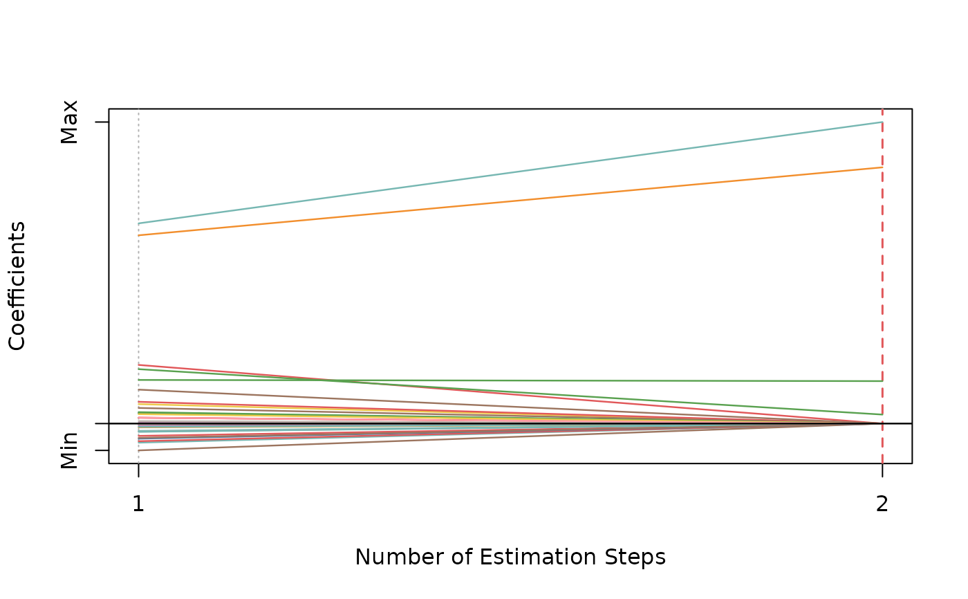
plot(asnet.fit)