Poor Man’s Neural Collaborative Filtering

We will use the simple SVD idea popularized by the Netflix prize. Let’s say we have a m x n matrix R with binary values r_{ui}. We want to decompose it into a m x k matrix P and a k x n matrix Q with k latent factors each. The inner product p_u x q_i derived by latent representations p_u and q_i from P and Q will be used to predict r_{ui}. Everything is differentiable here so it can be optimized by gradient descent methods.

Some modifications for dealing with the binary implicit feedback data:

• Since r_{ui} is binary (0-1 valued), we will use the binary cross entropy loss (commonly used for classification) instead of the regression-oriented MSE losses.
• As a remedy for the sparsity (or unbalanced classes) often presented in matrix R, we assign more weight to the less presented class (known interactions), which is necessarily “cost-sensitive learning”. Another possibility is to use random sampling to get different, much smaller sets of negative samples to balance the training data for each batch.
• The inner product layer or the part before it is easily replaceable by arbitrary DNN architectures. I didn’t do it here though because I prefer to keep the model simple.

As a reference, what we are trying to do here is similar to what He et al. (WWW 2017) proposed, but even more straightforward. I call it “poor man’s neural collaborative filtering”.

Applications to Quantitative Systems Pharmacology

Let’s try this model with our data. The dataset is from a statistical methodology paper we published in 2015. It contains 746 drugs and 817 adverse drug reactions (ADRs), with 24,803 known drug-ADR associations. This data can be represented by a 746 x 817 matrix with 0-1 entries, where 1 denotes for having a known association. It’s implicit feedback: we don’t know any non-association drug-ADR pairs here, and all the missing drug-ADR pairs (all the pairs other than the known associated pairs) are marked as 0. We are interested in predicting if there are any novel associations between all the missing drug-ADR pairs. If successful, we will be able to forecast if a specific drug has any potential but unreported side effects, which helps the clinical pharmacology and pharmacovigilance practice.

For our data, the model parameters are summarized below (only 15k parameters, yay):

_______________________________________________________________________________
Layer (type)                  Output Shape      Param #     Connected to
===============================================================================
input_1 (InputLayer)            (None, 1)         0
_______________________________________________________________________________
input_2 (InputLayer)            (None, 1)         0
_______________________________________________________________________________
embedding_1 (Embedding)       (None, 1, 10)       7460      input_1[0][0]
_______________________________________________________________________________
embedding_2 (Embedding)       (None, 1, 10)       8170      input_2[0][0]
_______________________________________________________________________________
flatten_1 (Flatten)             (None, 10)        0         embedding_1[0][0]
_______________________________________________________________________________
flatten_2 (Flatten)             (None, 10)        0         embedding_2[0][0]
_______________________________________________________________________________
dot_1 (Dot)                     (None, 1)         0         flatten_1[0][0]
                                                            flatten_2[0][0]
_______________________________________________________________________________
dense_1 (Dense)                 (None, 1)         2         dot_1[0][0]
===============================================================================
Total params: 15,632
Trainable params: 15,632
Non-trainable params: 0
_______________________________________________________________________________

Code and Results

Let’s code it up with R + Keras and train it on GPU:

The key parameters to tune here are:

• The optimizer. We chose RMSProp since it gave us the most stable training results.
• The number of latent factors k. We finally decided to use 5 because it is unlikely that one needs 50 factors to do this well. One probably also needs more layers for a larger k.
• The class_weight. We tried a few from 1:1 to 500:1 and finally selected the 50:1 ratio.
• The batch_size. Due to the sparsity of the matrix, this affects the performance.

The loss and accuracy changes in each epoch are visualized below:

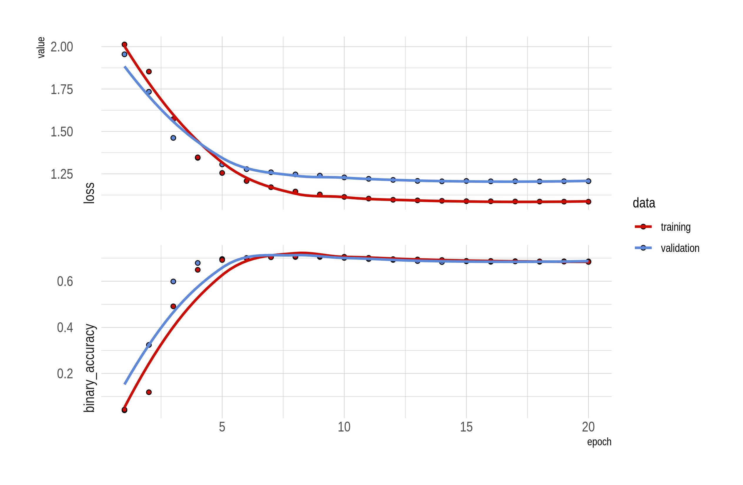
Figure: Converges within 10 epochs (after some slight tuning). The accuracy is around 0.7.

Comments

We have just prototyped a recommender system with only a few lines of R code, thanks to the flexibility offered by a modern machine learning framework with automatic differentiation and off-the-shelf optimizers. Two interesting topics to explore:

• Model architecture. The barebone model here is easily extensible to build hybrid recommender systems as we did in our 2015 paper. Such extensions can be defined as feature-based matrix factorization, meaning we can further incorporate features for the drugs and ADRs to improve the predictive performance. One can simply put them in a neural net architecture and let them play together with the latent factors learned here.
• Loss function. It is possible to try more loss functions, such as the triplet loss designed explicitly for one-class classification or metric learning problems.

Here is the GitHub repo for the R code.