Joint Power Analysis for Non-Symmetric Two-Stage Case-Control Designs
Source:vignettes/cats.Rmd
cats.RmdSource: http://www.popgen.dk/software/index.php/CATS
A simple run
library("cats")

cats(
  freq = 0.2,
  ncases = 500, ncases2 = 500,
  ncontrols = 1000, ncontrols2 = 1000,
  risk = 1.5, multiplicative = 1
)
#> Expected Power is;
#>
#>
#>
#>                    For a one-stage study = 0.94
#>       For first stage in two-stage study = 0.972
#> For second stage in replication analysis = 0.784
#>     For second stage in a joint analysis = 0.929
#>                                       pi = 0.5
Plot examples
Which design is better
rr <- seq(1, 2, by = 0.05)
maf <- c(0.05, 0.1, 0.2, 0.5)
c2 <- curve.cats(rr, maf,
  ncases = 600, ncontrols = 600, ncases2 = 600,
  ncontrols2 = 600, alpha = 0.000001, prevalence = 0.01
)
#> 1  2  3  4
plot(c2, type = "One", main = "power2", ylab = "Power", xlab = "RR", file = NULL, col = 1:4)
lines.cats(c2, type = "Replication", lty = 3)
lines.cats(c2, type = "Joint", lty = 2)
lines.cats(c2, type = "First", lty = 4)
legend("left", c("One stage", "Joint", "Relication", "First Stage"), lty = 1:4, bty = "n")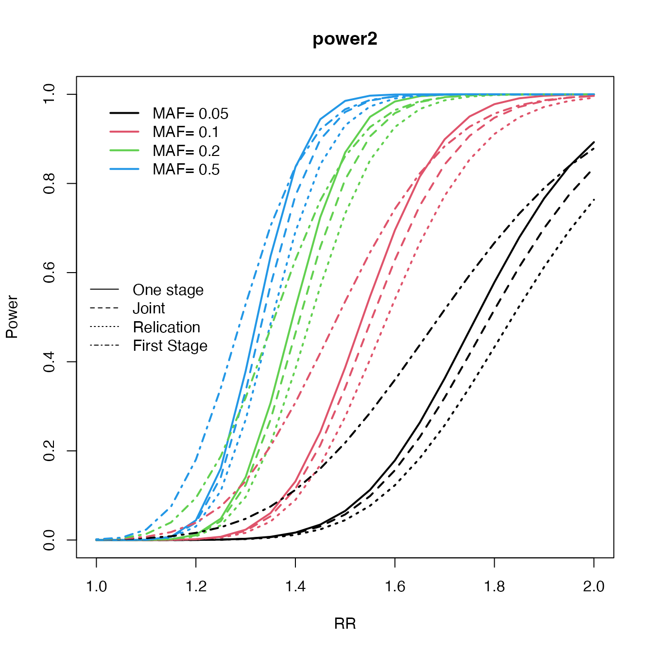
Number of SNPs for replication
power.J96 <- c()
power.J1536 <- c()
RR <- seq(1.1, 1.5, by = 0.025)
maf <- c(5, 10, 20, 50) / 100

for (tal2 in 1:length(maf)) {
  J1 <- c()
  J2 <- c()
  for (tal in 1:length(RR)) {
    temp <- cats(
      freq = maf[tal2], ncases = 1500, ncontrols = 1500, ncases2 = 2000,
      ncontrols2 = 2000, risk = RR[tal], pimarkers = 96 / 300000, alpha = 0.05 / 300000
    )
    J1[tal] <- temp$P.joint
    temp <- cats(
      freq = maf[tal2], ncases = 1500, ncontrols = 1500, ncases2 = 2000,
      ncontrols2 = 2000, risk = RR[tal], pimarkers = 1536 / 300000, alpha = 0.05 / 300000
    )
    J2[tal] <- temp$P.joint
  }
  power.J96 <- cbind(power.J96, J1)
  power.J1536 <- cbind(power.J1536, J2)
}
col <- 1:length(maf)

plot(RR, power.J1536[, 1], type = "l", lwd = 2, ylab = "Power", main = "Multiplicative model,
 1500:1500, 2000:2000", col = col[1], ylim = 0:1)
for (tal2 in 2:length(maf)) lines(RR, power.J1536[, tal2], lwd = 2, col = col[tal2], type = "l")
for (tal2 in 1:length(maf)) lines(RR, power.J96[, tal2], lwd = 2, col = col[tal2], type = "l", lty = 2)
legend("bottomright", c(paste("MAF=", c(maf), ", rep=1536"), paste("MAF=", c(maf), ", rep=96")), col = col, lwd = 2, bty = "n", lty = c(rep(1, length(maf)), rep(2, length(maf))))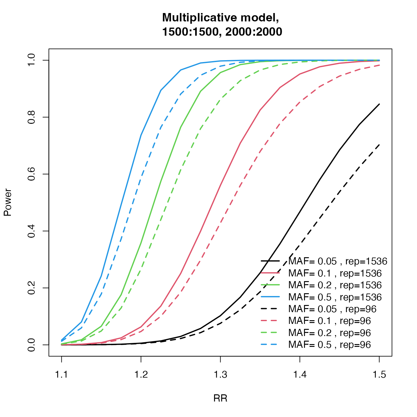
Heatmap of power
rr <- seq(1, 2, by = 0.025)
c <- super.cats(rr,
  by = length(rr), ncases = 765, ncontrols = 1274, ncases2 = 100, ncontrols2 = 100,
  alpha = 0.001, prevalence = 0.01
)
#> 1  2  3  4  5  6  7  8  9  10  11  12  13  14  15  16  17  18  19  20  21  22  23  24  25  26  27  28  29  30  31  32  33  34  35  36  37  38  39  40  41  42
plot(c, main = "power", file = NULL)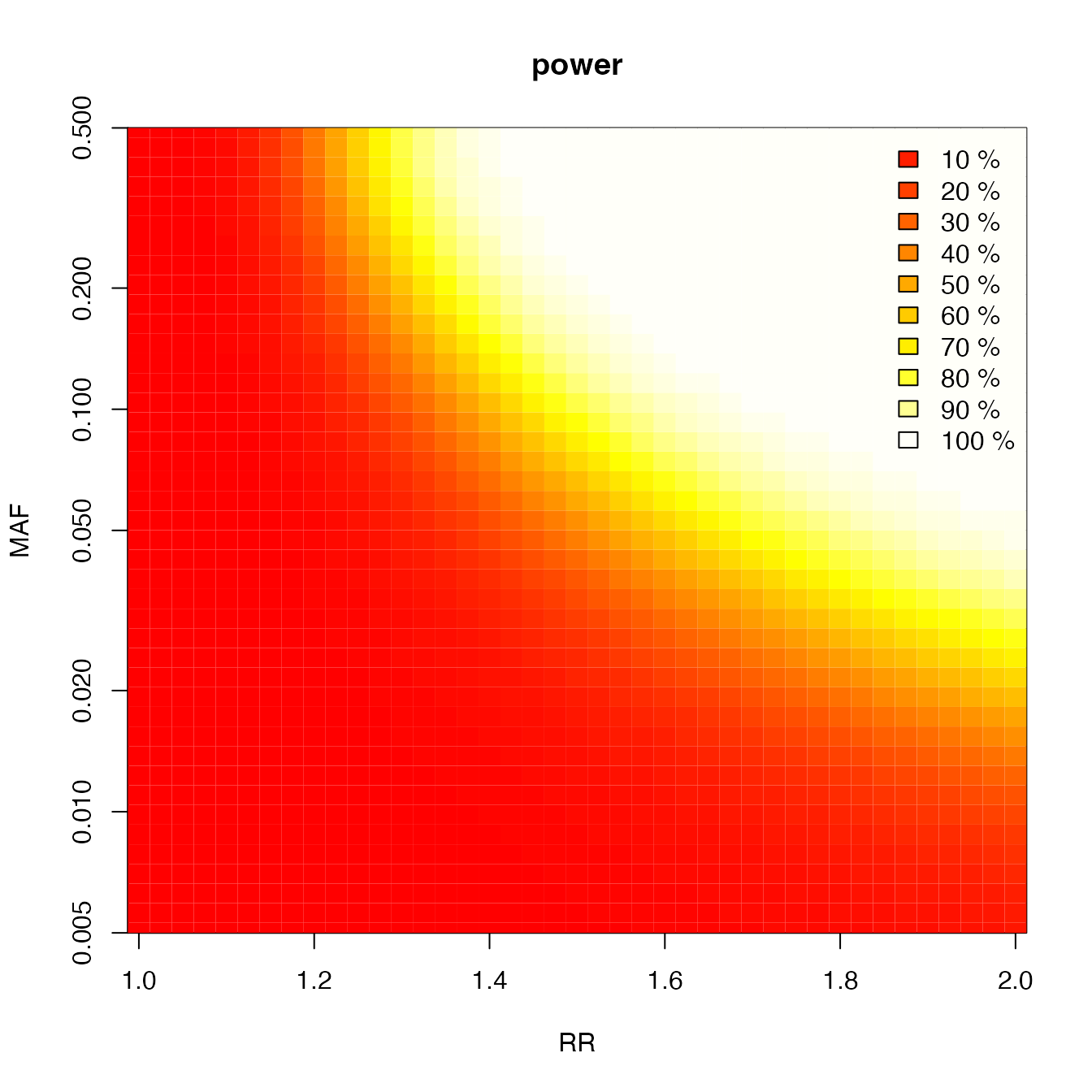
Design and MAF
rr <- seq(1, 2, by = 0.05)
maf <- c(0.05, 0.1, 0.2, 0.5)
c2 <- curve.cats(rr, maf,
  ncases = 600, ncontrols = 600, ncases2 = 600, ncontrols2 = 600,
  alpha = 0.000001, prevalence = 0.01
)
#> 1  2  3  4

plot(c2, type = "One", main = "power2", ylab = "Power", xlab = "RR", file = NULL, col = 1:4)
lines.cats(c2, type = "Replication", lty = 3)
lines.cats(c2, type = "Joint", lty = 2)
lines.cats(c2, type = "First", lty = 4)
legend("left", c("One stage", "Joint", "Relication", "First Stage"), lty = 1:4, bty = "n")