msaenet 3.1.2 and a sparse survival modeling example

I’m pleased to announce that msaenet 3.1.2 is now available on CRAN.
You can install msaenet with:
install.packages("msaenet")If you frequently build sparse linear models, msaenet can help you generate more parsimonious solutions with adaptive estimations. It supports any number of adaptive estimation steps, flexible initialization methods, multiple model selection criteria, and automatic parallel parameter tuning.
New color palette
This is a more focused update compared to the 3.1.1 update in March 2024. The main user-visible change is the new default color palette (new Tableau 10) now used for the coefficient profile plot.

Figure 1: Default color palettes: old (top) vs. new (bottom).
The new palette has a softer tone, potentially improving accessibility for users with color vision deficiencies. This color palette is also applied to all plot types, as seen in the example below.
High-dimensional survival analysis example
Here, we use a simulated dataset with high-dimensional covariates and survival outcomes to show how msaenet works and compare it with classic models.
library("msaenet")First, we create a function to generate simulated data. The idea is borrowed directly from glmnet::Cindex(). It is straightforward and does not consider factors such as correlation structure or signal strength/noise level.
sim_cox <- function(n, p, p_nzv, p_train) {
  x <- matrix(rnorm(n * p), nrow = n, ncol = p)

  nzc <- p * p_nzv
  beta <- rnorm(nzc)
  fx <- x[, seq(nzc)] %*% beta / 3
  hx <- exp(fx)
  ty <- rexp(n, hx)
  tcens <- rbinom(n, prob = 0.3, size = 1)
  y <- survival::Surv(ty, event = 1 - tcens)

  idx_tr <- sample(seq(n), size = round(n * p_train))
  idx_te <- setdiff(seq(n), idx_tr)
  x_tr <- x[idx_tr, , drop = FALSE]
  y_tr <- y[idx_tr, , drop = FALSE]
  x_te <- x[idx_te, , drop = FALSE]
  y_te <- y[idx_te, , drop = FALSE]

  list("x_train" = x_tr, "y_train" = y_tr, "x_test" = x_te, "y_test" = y_te)
}
Next, we use the function to generate a training set with 1,000 observations and an independent test set with 1,000 observations. The number of variables is 2,000, among which only 2.5% (50) are “true” variables with non-zero coefficients. This makes it a sparse regression problem.
set.seed(42)
sim_data <- sim_cox(n = 2000, p = 2000, p_nzv = 0.025, p_train = 0.5)
Then we fit an msaenet model with basic setups:
- Initialization: ridge regression.
- \(\alpha\) tuning grid: 0.05 to 0.95, with step size 0.05.
- Parameter tuning for each estimation step: 5-fold cross-validation.
- Maximum number of adaptive estimation steps: 10.
- Optimal step number selection: Bayesian information criterion.
doParallel::registerDoParallel(parallelly::availableCores())

fit_msaenet <- msaenet(
  sim_data$x_train,
  sim_data$y_train,
  family = "cox",
  init = "ridge",
  alphas = seq(0.5, 0.95, 0.05),
  tune = "cv",
  nfolds = 5L,
  rule = "lambda.1se",
  nsteps = 10L,
  tune.nsteps = "bic",
  seed = 42,
  parallel = TRUE,
  verbose = FALSE
)
We generate a coefficient profile plot where the x-axis shows the estimation step, and y-axis shows how each coefficient changes across all steps. The optimal step is highlighted with a vertical red dashed line by default.
plot(fit_msaenet)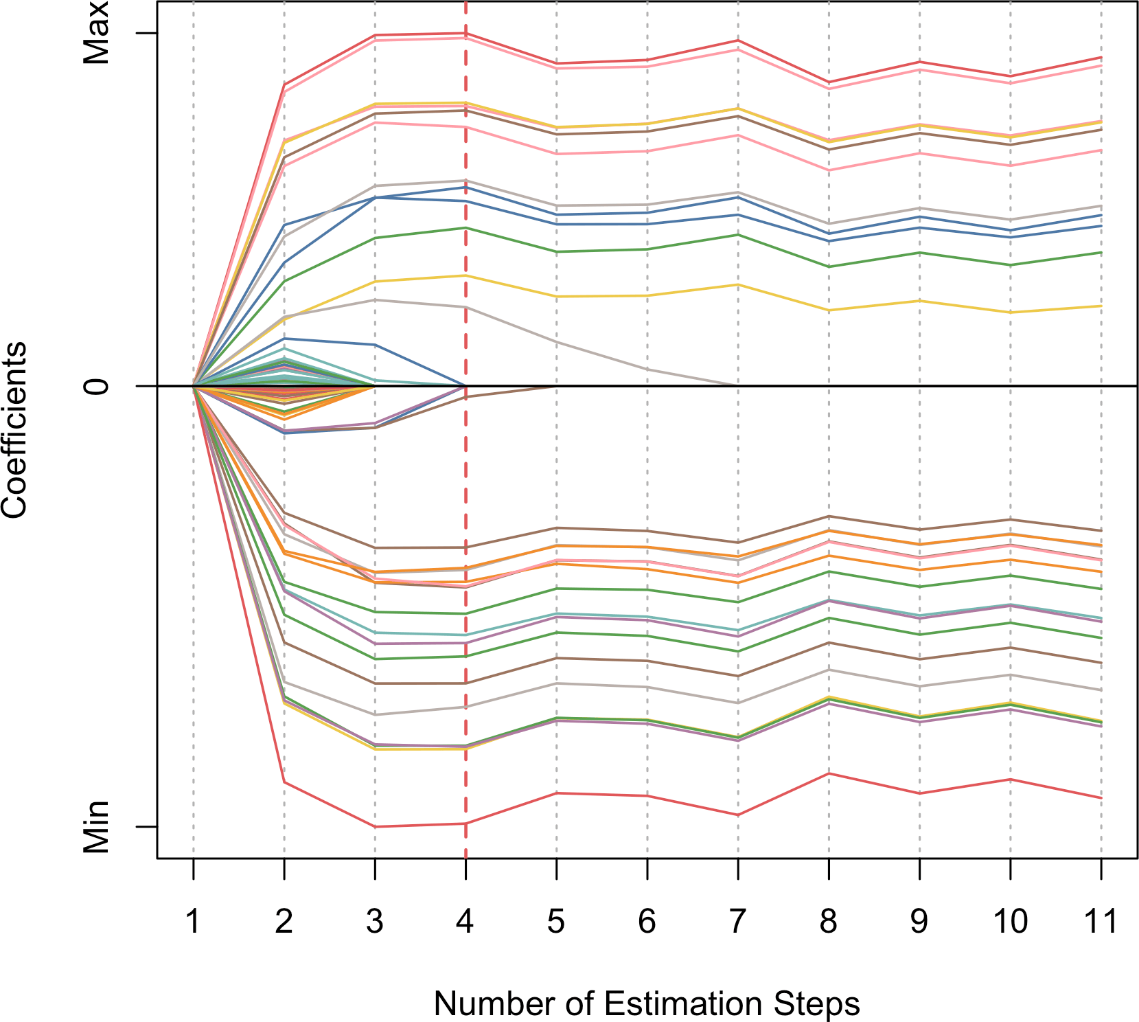
Figure 2: Coefficient profile plot showing coefficient changes through adaptive estimation steps.
Switching to type = "criterion" creates a scree plot that shows how the
model selection criterion (BIC here) changes in each step.
plot(fit_msaenet, type = "criterion")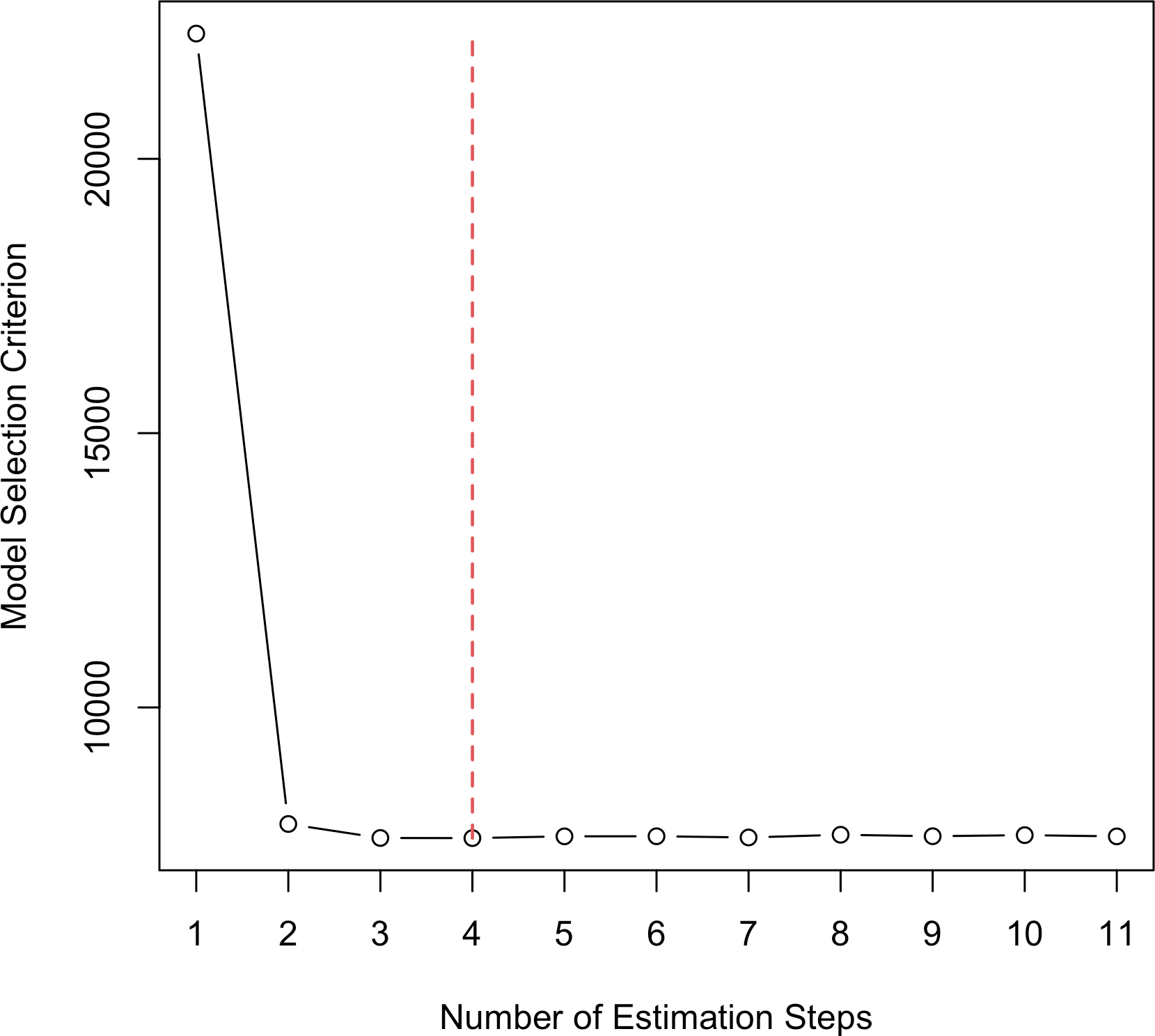
Figure 3: Scree plot showing BIC changes through adaptive estimation steps.
Using type = "dotplot" produces a dot plot showing the “optimal” model
coefficients with various
variable labeling options
available.
plot(fit_msaenet, type = "dotplot", label = TRUE)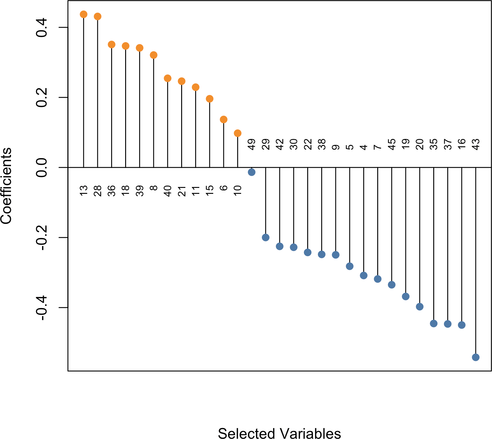
Figure 4: Dot plot showing the non-zero coefficients from the optimal model.
We evaluate the number of true positive, false positive, and false negative selections. We also calculate the concordance index (C-index) on the training set and the independent test set.
idx_nzv <- 1L:(2000 * 0.025)

msaenet.tp(fit_msaenet, true.idx = idx_nzv)
#> [1] 29
msaenet.fp(fit_msaenet, true.idx = idx_nzv)
#> [1] 0
msaenet.fn(fit_msaenet, true.idx = idx_nzv)
#> [1] 21

glmnet::Cindex(
  as.vector(predict(fit_msaenet, newx = sim_data$x_train)),
  y = sim_data$y_train
)
#> [1] 0.8431152
glmnet::Cindex(
  as.vector(predict(fit_msaenet, newx = sim_data$x_test)),
  y = sim_data$y_test
)
#> [1] 0.8403838
For comparison, we fit a lasso and a “canonical” elastic-net model (\(\alpha = 0.5\)) with glmnet. An adaptive elastic-net model is available from the fitted msaenet model.
doParallel::registerDoParallel(parallelly::availableCores())

cv_lasso <- glmnet::cv.glmnet(
  sim_data$x_train,
  sim_data$y_train,
  nfolds = 5,
  family = "cox",
  alpha = 1,
  parallel = TRUE
)

fit_lasso <- glmnet::glmnet(
  sim_data$x_train,
  sim_data$y_train,
  family = "cox",
  alpha = 1,
  lambda = cv_lasso$lambda.1se
)

cv_enet <- glmnet::cv.glmnet(
  sim_data$x_train,
  sim_data$y_train,
  nfolds = 5,
  family = "cox",
  alpha = 0.5,
  parallel = TRUE
)

fit_enet <- glmnet::glmnet(
  sim_data$x_train,
  sim_data$y_train,
  family = "cox",
  alpha = 0.5,
  lambda = cv_enet$lambda.1se
)

fit_aenet <- fit_msaenet$model.list[[2]]
We create a few utility functions for computing the same evaluation metrics used above: TP, FP, FN for variable selection, C-index for predictive performance.
glmnet.nzv <- function(object) {
  which(abs(as.vector(object$beta)) > .Machine$double.eps)
}

glmnet.tp <- function(object, true.idx) {
  length(intersect(glmnet.nzv(object), true.idx))
}

glmnet.fp <- function(object, true.idx) {
  length(setdiff(glmnet.nzv(object), true.idx))
}

glmnet.fn <- function(object, true.idx) {
  length(setdiff(true.idx, glmnet.nzv(object)))
}

metrics <- function(object, true.idx, data) {
  if (inherits(object, "msaenet")) {
    tp <- msaenet.tp(object, true.idx = true.idx)
    fp <- msaenet.fp(object, true.idx = true.idx)
    fn <- msaenet.fn(object, true.idx = true.idx)
  }
  if (inherits(object, "glmnet")) {
    tp <- glmnet.tp(object, true.idx = true.idx)
    fp <- glmnet.fp(object, true.idx = true.idx)
    fn <- glmnet.fn(object, true.idx = true.idx)
  }
  cindex_train <- glmnet::Cindex(
    as.vector(predict(object, newx = data$x_train)),
    y = data$y_train
  )
  cindex_test <- glmnet::Cindex(
    as.vector(predict(object, newx = data$x_test)),
    y = data$y_test
  )
  c(
    "TP" = tp,
    "FP" = fp,
    "FN" = fn,
    "C-index train" = format(round(cindex_train, 4), nsmall = 4),
    "C-index test" = format(round(cindex_test, 4), nsmall = 4)
  )
}
Summarizing all model metrics in a table:
df <- rbind(
  "lasso"   = metrics(fit_lasso,   idx_nzv, sim_data),
  "enet"    = metrics(fit_enet,    idx_nzv, sim_data),
  "aenet"   = metrics(fit_aenet,   idx_nzv, sim_data),
  "msaenet" = metrics(fit_msaenet, idx_nzv, sim_data)
)

knitr::kable(
  df,
  align = rep("r", 5),
  format = "html",
  table.attr = "class=\"table table-hover\""
)| TP | FP | FN | C-index train | C-index test | |
|---|---|---|---|---|---|
| lasso | 38 | 89 | 12 | 0.8633 | 0.8392 |
| enet | 34 | 63 | 16 | 0.8538 | 0.8341 |
| aenet | 32 | 37 | 18 | 0.8514 | 0.8374 |
| msaenet | 29 | 0 | 21 | 0.8431 | 0.8404 |
We were able to reduce the number of false positive selections from 89 down to 0, with a trade-off of selecting 9 fewer true variables. For this particular simulated dataset, with fewer variables selected, the C-index was not affected and even slightly improved on the independent test set.
From the initial experimental results, we see that msaenet likely prioritizes precision (minimizing false positive selections) over recall (maximizing true positive selections). While this may not be ideal, it could be useful, especially in scenarios where the costs of false positive selections outweigh the costs of false negative selections, and precision is the priority.
How to cite msaenet
If you find msaenet useful, you can cite it as follows:
Nan Xiao and Qing-Song Xu. (2015). Multi-step adaptive elastic-net: reducing false positives in high-dimensional variable selection. Journal of Statistical Computation and Simulation 85(18), 3755–3765.
A BibTeX entry for LaTeX users is:
@article{xiao2015multi,
  title   = {Multi-step adaptive elastic-net:
             reducing false positives in high-dimensional variable selection},
  author  = {Nan Xiao and Qing-Song Xu},
  journal = {Journal of Statistical Computation and Simulation},
  volume  = {85},
  number  = {18},
  pages   = {3755--3765},
  year    = {2015},
  doi     = {10.1080/00949655.2015.1016944}
}