ggsci 3.2.0: new color palettes from Observable, Bootstrap, and Tailwind CSS
I am delighted to announce the release of ggsci 3.2.0. The R package ggsci was first released in 2016. It offers a range of ggplot2 color scales drawn from various sources, including scientific publications, data visualization tools, sci-fi movies, and television series.
To install ggsci from CRAN, use:
install.packages("ggsci")As a follow-up to the ggsci 3.1.0 release, ggsci 3.2.0 introduces three new color scales and continues to improve the package engineering details.
Observable 10
The Observable 10 palette was officially announced in April 2024. It was designed as the new default categorical color scheme for Observable Plot, the JavaScript library for tabular data visualization. To me, this new color palette offers a fresh and clean aesthetic while maintaining accessibility and robustness for data visualization purposes.
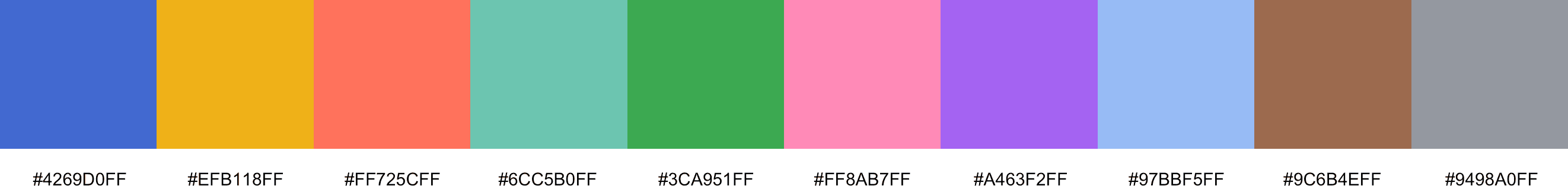
Figure 1: The Observable 10 palette added in ggsci 3.2.0.
In ggsci, this palette is made available via the new color scale functions
scale_color_observable() and scale_fill_observable().
Here is a ggplot2 example that uses this color palette to visualize five categories.
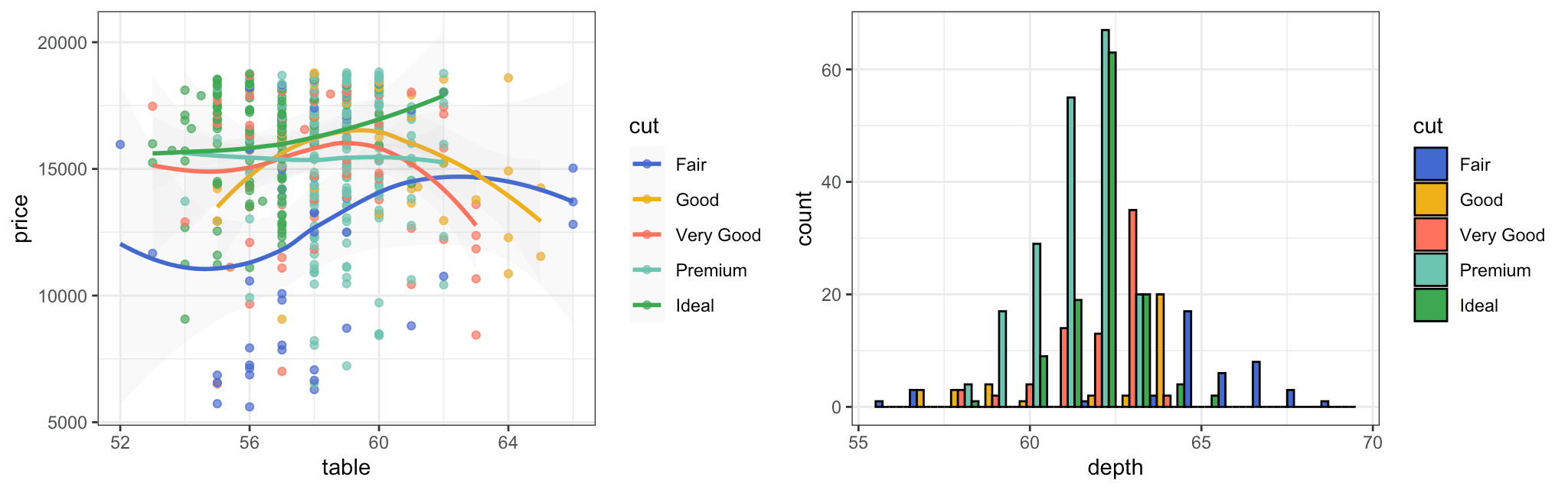
Figure 2: ggplot2 example using the Observable 10 color scales.
Bootstrap and Tailwind CSS palettes
It has been quite a while since we expanded continuous color scales in ggsci. For a new start, I have chosen to implement the default color systems from Bootstrap 5 and Tailwind CSS 3, the two most popular front-end frameworks. These palettes have been refined over years of development, making them possible choices for data visualization.
Using ColorBrewer’s terminology, these color systems contain multiple single-hue sequential color schemes. They are suitable for representing values in ordered or numeric data, such as heatmap visualizations.
In ggsci, these are made available via
scale_color_bs5()/scale_fill_bs5()
and scale_color_tw3()/scale_fill_tw3().
We can easily visualize them using
colorspace::swatchplot().
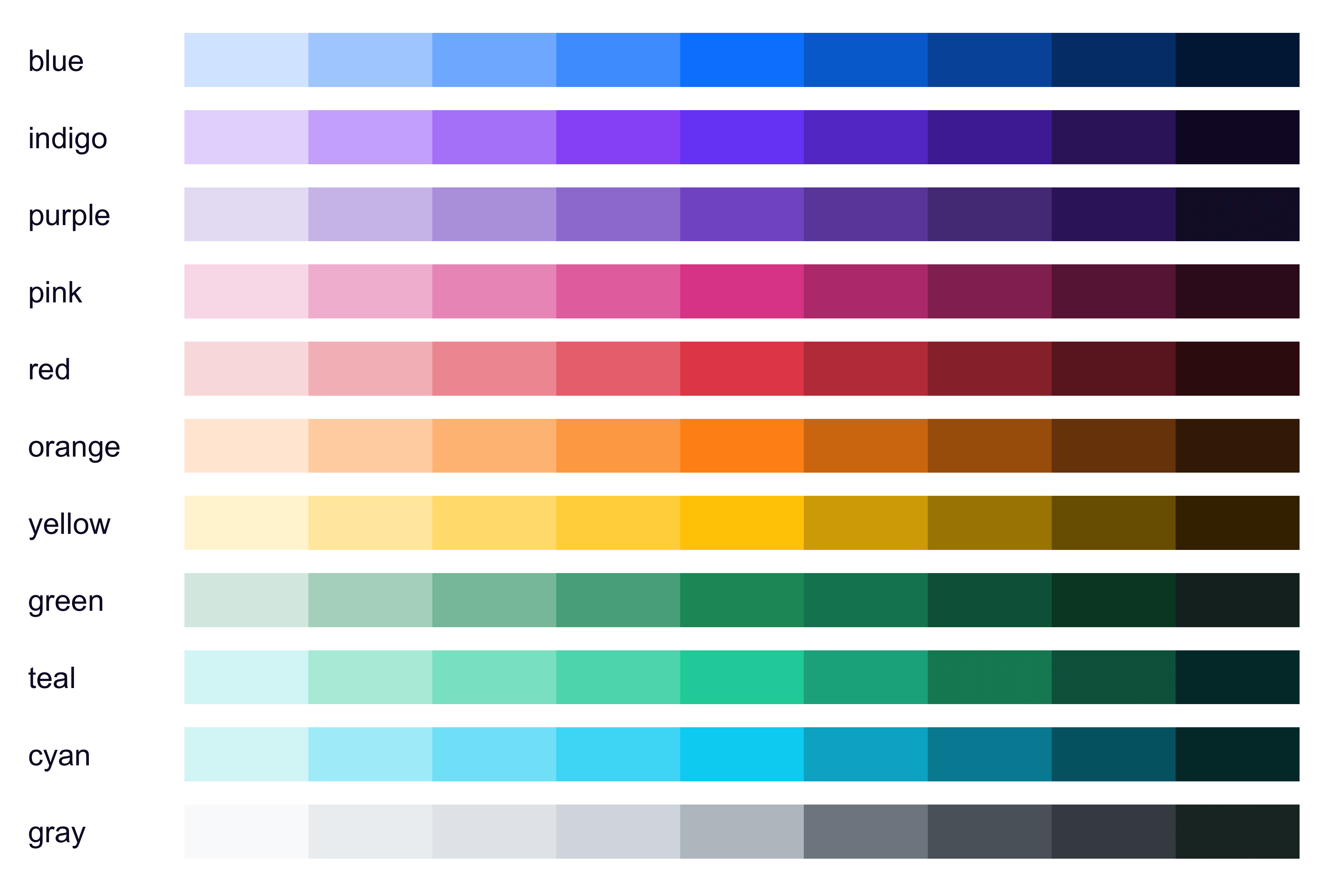
Figure 3: The 11 Bootstrap 5 continuous palettes added in ggsci 3.2.0.
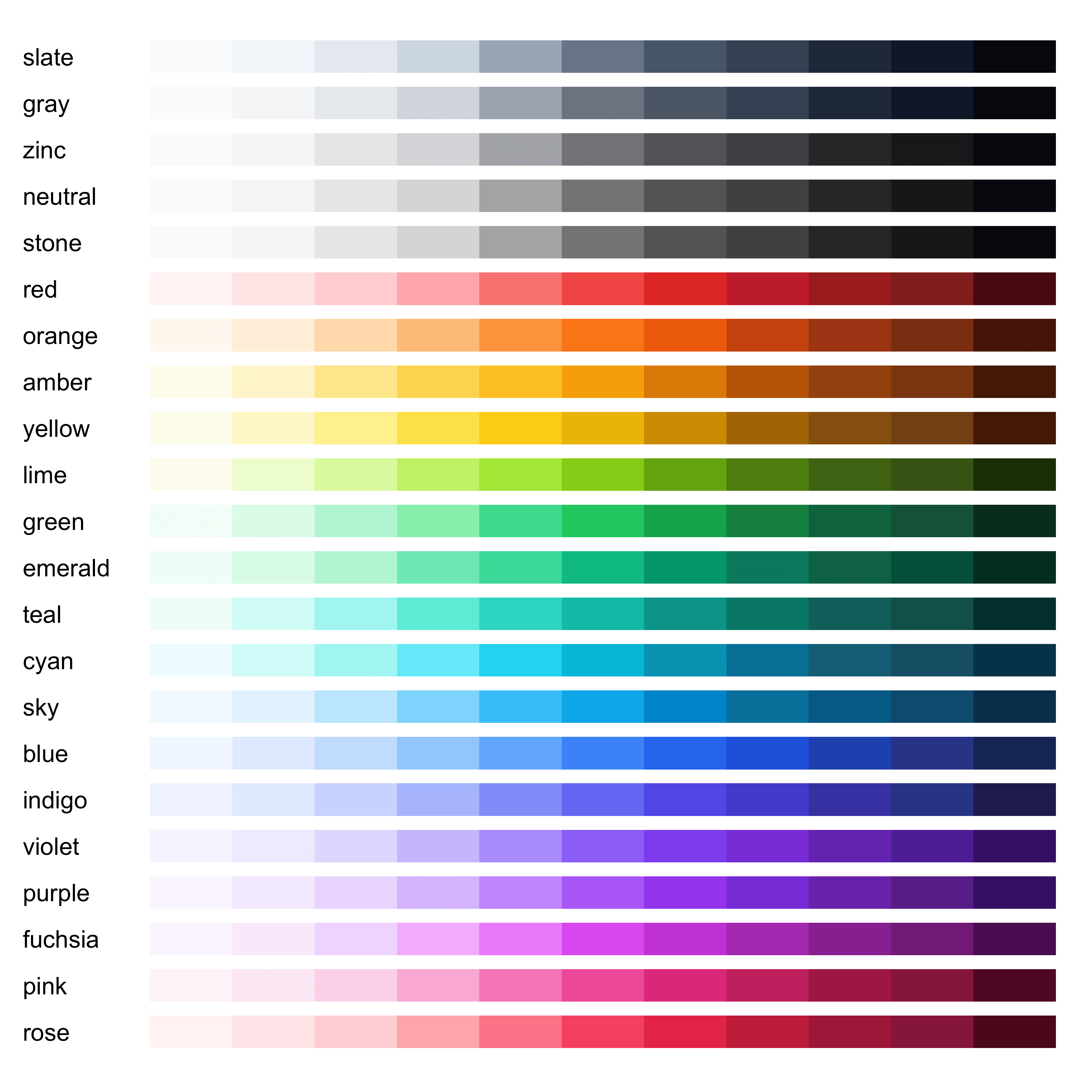
Figure 4: The 22 Tailwind CSS continuous palettes added in ggsci 3.2.0.
Other improvements
As the package grows, it is even more important to keep things light so that we have enough space to expand to even more color scales comfortably.
I first
moved the internal color palette data
out of the binary file R/sysdata.rda and moved it into R/palettes.R instead.
This change makes everything plain text
(which is unreasonably effective).
I hope this simplifies third-party contributions by eliminating the
tedious .rda file generation step with the previous R script in data-raw/.
The other set of optimizations was applied to the continuous color scale code examples. Besides removing the soft dependency reshape2 from the code, I fine-tuned the layout with a more compact grid to reduce the output image size in #46, reducing the package size concerns described in the previous post.
What’s next?
I’m open to new ideas on the next color palettes to add. If you have a suggestion, please submit them by creating an issue.