Bayesian Lasso with greta
The R code to reproduce the results is available from GitHub Gist.

Although I am not an expert in Bayesian statistics, I always have an idealized version of the framework for Bayesian modeling in my mind:
- Allows defining data models intuitively — preferably in native R.
- Handles the low-level computations such as MCMC automatically.
- Works on both CPU and GPU seamlessly would be perfect for 2020.
All these features would help me focus on the task instead of the tool better. Among others, Stan and Edward were pretty close to achieving these goals.
Created by Professor Nick Golding, greta is now my all-time favorite. It has all the traits described above. You can see this from its example models. To know it better, I experimented with it a bit for fitting Bayesian sparse regression models. I soon realized the simplicity provided by greta could truly enable fast exploration of modeling strategies for a range of problems.
Generate synthetic data
Under the linear model \(y = X \beta + \varepsilon\), we will generate 1000 samples: use 500 for fitting the model and leave the rest 500 as the independent test set. The first 10 variables in the total 1000 variables have a non-zero coefficient. A moderate correlation exists between variables. The signal-to-noise ratio (SNR) is also moderate. We simulate the data with msaenet:
library("msaenet")

n <- 500
p <- 1000
pnz <- 10

dat <- msaenet.sim.gaussian(
  n = n * 2, p = p,
  rho = 0.5, coef = rep(5, pnz), snr = 3,
  p.train = 0.5, seed = 42
)

x <- dat$x.tr
y <- dat$y.tr
beta <- c(rep(5, pnz), rep(0, p - pnz))
Note: this is for illustrating the modeling processes only. It is not a comprehensive benchmark in any way. Under many other settings and parameter tuning methods, the results can be very different.
Multi-step adaptive elastic-net
Let’s fit a msaenet model to check if things work, since it offers a look into a pool of models with \(\ell_1\) + \(\ell_2\) regularizations:
fit_msaenet <- msaenet(
  x, y,
  family = "gaussian",
  init = "ridge", alphas = seq(0.05, 0.95, 0.05),
  tune = "cv", nfolds = 10, rule = "lambda.min",
  nsteps = 20, tune.nsteps = "ebic"
)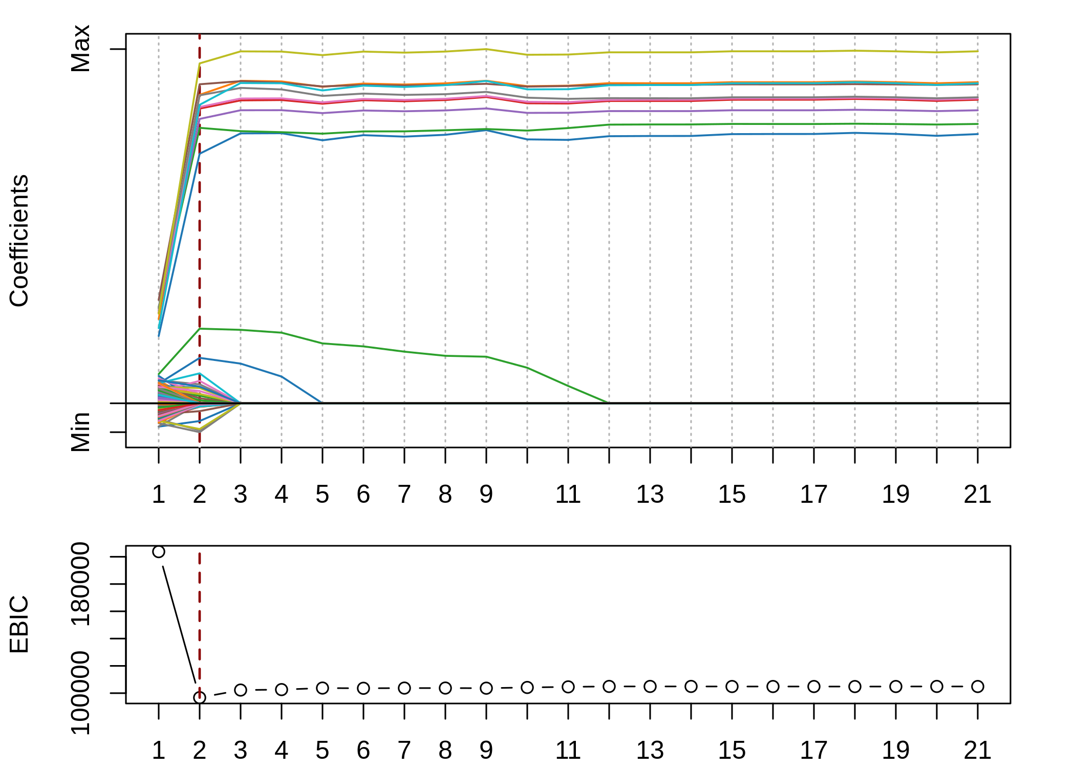
We achieved the lowest EBIC in step 2, which is equivalent to an adaptive elastic-net model. We selected 36 variables in total: all the 10 true variables and 26 false positive variables. The MSE is 203.
Lasso
Fit an ordinary lasso model with glmnet:
library("glmnet")

cv_lasso <- cv.glmnet(x, y, family = "gaussian", alpha = 1, nfolds = 10)
fit_lasso <- glmnet(x, y, family = "gaussian", alpha = 1, lambda = cv_lasso$lambda.min)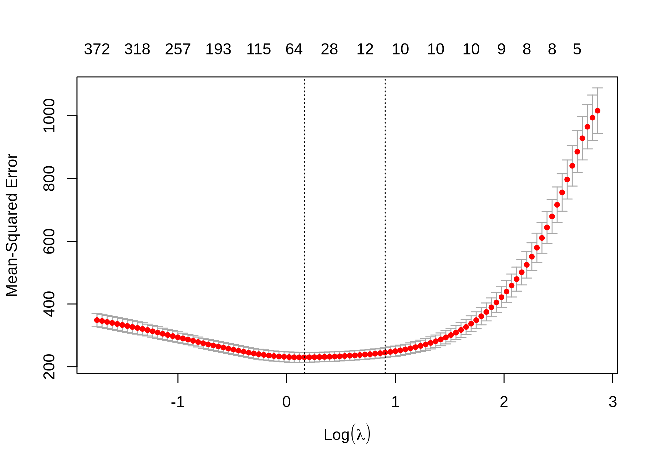
The model selected 56 variables in total: all the 10 true variables and 46 false positive variables. The MSE is 202.
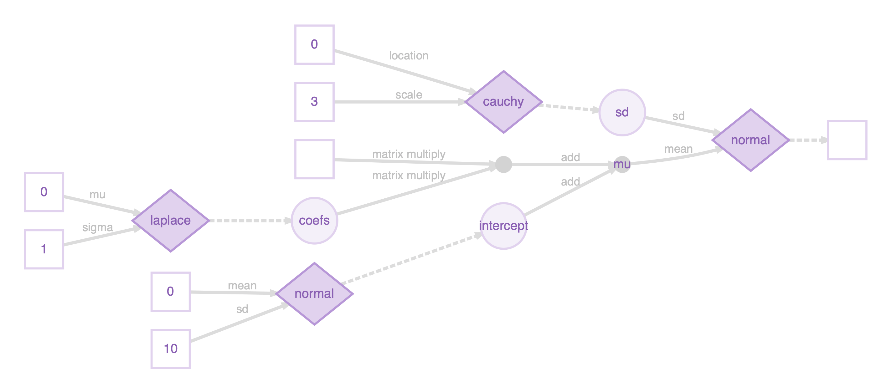
Bayesian Lasso
Define a Bayesian lasso model using the Laplace prior in greta:
library("greta")

intercept <- normal(0, 10)
sd <- cauchy(0, 3, truncation = c(0, Inf))
coefs <- laplace(0, 1, dim = ncol(x))
mu <- intercept + x %*% coefs
distribution(y) <- normal(mu, sd)

m <- model(intercept, coefs, sd)

draws_blasso <- mcmc(m, warmup = 1000, n_samples = 5000, chains = 8)
The computational graph by plotting m:
Plot the posterior mean and 95% credible interval of the coefficients:
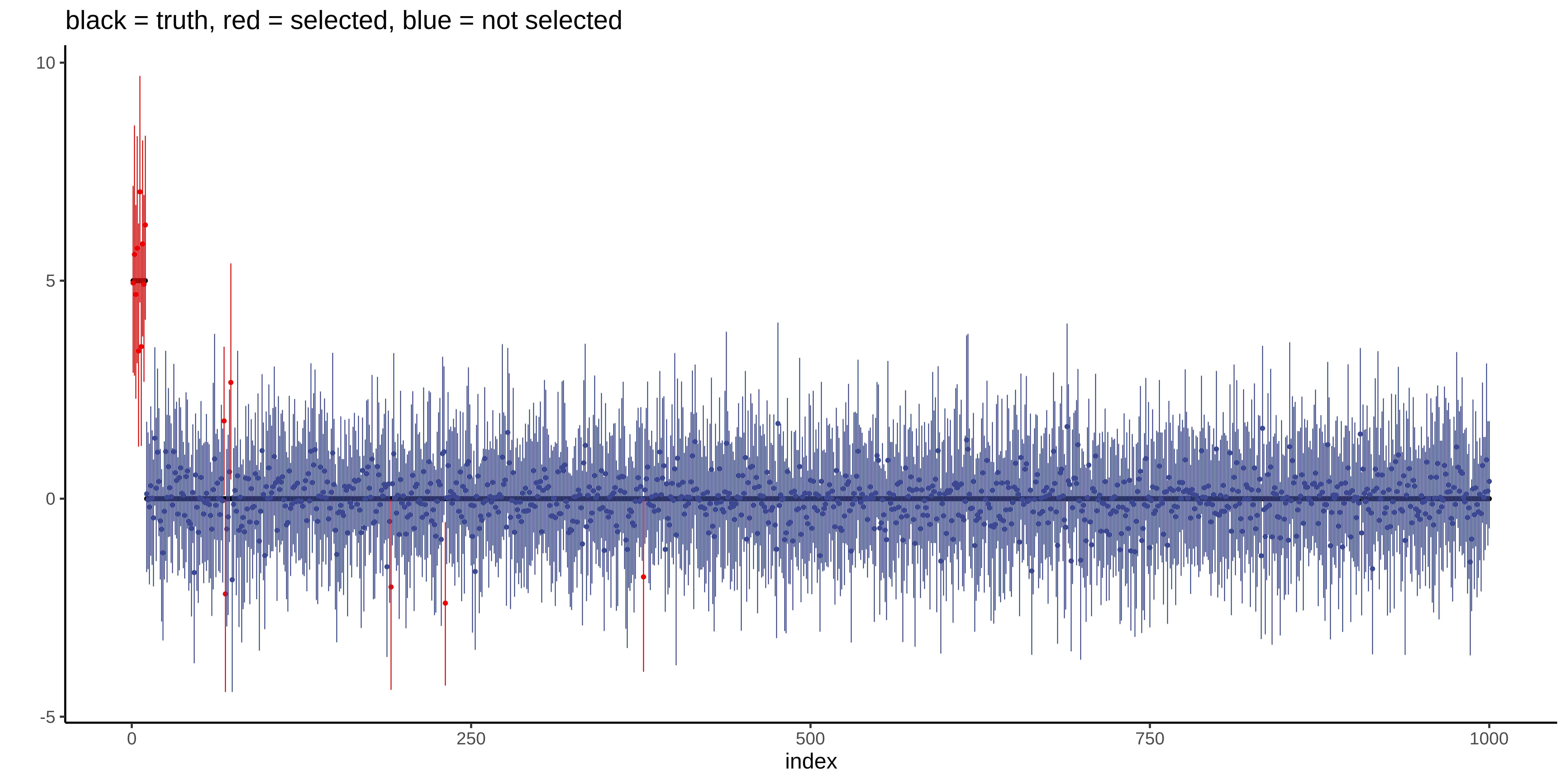
The model selected 16 variables: all the 10 true variables with 6 false positive variables. The MSE is 217.
For more theoretical discussions and empirical comparisons on Bayesian sparse shrinkage in regression, I find the notes from Jeffrey Arnold and Michael Betancourt useful. To me, it is still a bit magical how intuitively the lasso and Bayesian lasso are connected. I like this type of connection.
Summary
All three methods correctly selected all the true variables (TP). Regarding the number of false positive variables (FP) and MSE:
- msaenet: moderate MSE close to Lasso; moderate FP
- Lasso: smallest MSE close to msaenet; largest FP
- Bayesian lasso: largest MSE (not too bad though); smallest FP
| Method | TP | FP | MSE |
|---|---|---|---|
| msaenet | 10 | 26 | 203 |
| Lasso | 10 | 46 | 202 |
| Bayesian Lasso | 10 | 6 | 217 |
I would not read into this result too much as it only shows a small facet of the possible modeling approaches. It does demonstrate Bayesian Lasso’s potential and the flexibility of greta in probabilistic modeling. I would also try the more recent methods such as L0Learn and susieR in any real tasks as they offer some modern understanding of the problem.
By changing the cross-validation \(\lambda\) selection rule from lambda.min to lambda.1se in msaenet and lasso, you will be able to get models with 10 TP variables, 0 FP variables, and an even smaller MSE. It is not used above because I think the rule might introduce an extra “prior” in the Bayesian sense, thus not creating a fair comparison. Similarly, the Bayesian lasso model parameters can also be further tuned, including the priors and variable selection criteria.
I would love to hear your feedback. Please leave a note if you find me made a mistake somewhere or have some suggestions.