Table of Contents
Data Model
Let’s denote the vaccine-symptom pairs from the VAERS database as \(2 \times 2\) contingency tables:
| Target vaccine | Target symptom | All other symptoms | Total |
|---|---|---|---|
| Yes | \(n_{ij}\) | \(n_i - n_{ij}\) | \(n_i\) |
| No | \(n_j - n_{ij}\) | \(n - n_i - n_j + n_{ij}\) | \(n - n_i\) |
| Total | \(n_j\) | \(n - n_j\) | \(n\) |
It is often the case than not that \(n_{ij}\) occures as a rare event such that the observed count follows a Poisson distribution. In the GPS algorithm, we model the relative reporting ratio (RRR), which measures the ratio of how many symptoms under vaccine were actually observed over the number of expected symptoms, under the assumption that the symptoms and vaccine exposure are independent. The RRR (\(\lambda\)) is defined as
\[ \lambda_{ij} = \frac{\mu_{ij}}{E_{ij}}. \]
\(\mu_{ij}\) is the mean of the Poisson distribution of \(n_{ij}\). \(E_{ij}\) is the expected event count under the assumption that the vaccine exposure and the symptom are idependent. It can be estimated as
\[ \hat{E_{ij}} = \frac{n_i n_j}{n}. \]
For \(\lambda\), we can use a gamma distribution as a conjugate prior since the Poisson distributed \(n_{ij}\). (\(n_{ij} \sim Poisson (\mu_{ij})\)). In the GPS model, a simple mixture of two Gamma distributions was used as the prior to allow for more flexibility in the model:
\[ \lambda_{ij} \sim P \ \text{Gamma}(\alpha_1, \beta_1) + (1-P) \ \text{Gamma}(\alpha_2, \beta_2). \]
Using an empirical Bayesian approach, we can use the data to estimate the paramaters (\(\alpha_1\), \(\alpha_2\), \(\beta_1\), \(\beta_2\), \(P\)), calculate the posterior for \(\lambda\), and then derive the expectation of \(\log(\lambda)\):
\[ E(\log(\lambda)) = Q (\psi (\alpha_1 + n_{ij}) - \log(1/\beta_1 + E_{ij})) + (1-Q) (\psi (\alpha_2 + n_{ij}) - \log(1/\beta_2) + E_{ij}) \]
where
\[ Q = \frac{P \cdot \text{NB}(n_{ij}, E_{ij} \ | \ \alpha_1, \beta_1)}{P \cdot \text{NB}(n_{ij}, E_{ij} \ | \ \alpha_1, \beta_1) + (1-P) \cdot \text{NB}(n_{ij}, E_{ij} \ | \ \alpha_2, \beta_2)} \]
\(\psi\) is the digamma function. \(\text{NB}\) is the negative binomial distribution.
With the expectation of \(\log(\lambda)\), we can define the Empirical Bayesian Geometric Mean (EBGM) as
\[EBGM = e^{E(\log(\lambda))}.\]
The fifth percentile of the posterior distribution of \(\lambda\) is denoted as EB05 and interpreted as the lower one-sided 95% confidence limit for the EBGM. This estimator gives more conservative estimates when the event counts are small, thus yields a shrinkage estimate which could reduce the number of false-positive signals.
Calculate PRR
To fit a Gamma Poisson Shrinker model (DuMouchel 1999), we first calculate actual counts (N), expected counts (E) of each vaccine-symptom combination, relative reporting ratio (RRR), and proportional reporting ratio (PRR) using age + gender stratification to control potential confounding effects:
library("openEBGM")
library("magrittr")
library("kableExtra")
library("ggsci")

df_p <- readRDS("data-processed/df.rds") %>%
  processRaw(stratify = TRUE, zeroes = FALSE)
# stratification variables used: strat_age, strat_gender
# there were 12 strata:  <= 2-Female, <= 2-Male, <= 2-Unknown, > 65-Female, > 65-Male, > 65-Unknown, 18 - 65-Female, 18 - 65-Male, 18 - 65-Unknown, 2 - 18-Female, 2 - 18-Male, 2 - 18-Unknown
Sanity check:
df_p %>% head()
                        var1             var2 N           E     RR
1 ADENOVIRUS (NO BRAND NAME)       Arthralgia 1 0.119480157   8.37
2 ADENOVIRUS (NO BRAND NAME)         Dyspnoea 1 0.083668035  11.95
3 ADENOVIRUS (NO BRAND NAME)      Face oedema 1 0.011163701  89.58
4 ADENOVIRUS (NO BRAND NAME) Gait disturbance 1 0.014375342  69.56
5 ADENOVIRUS (NO BRAND NAME)   Osteoarthritis 1 0.005387014 185.63
6 ADENOVIRUS (NO BRAND NAME)        Petechiae 1 0.002717102 368.04
     PRR
1  16.26
2  17.43
3  86.42
4  67.12
5 296.72
6 212.56
#                         var1             var2 N           E     RR    PRR
# 1 ADENOVIRUS (NO BRAND NAME)       Arthralgia 1 0.119480157   8.37  16.26
# 2 ADENOVIRUS (NO BRAND NAME)         Dyspnoea 1 0.083668035  11.95  17.43
# 3 ADENOVIRUS (NO BRAND NAME)      Face oedema 1 0.011163701  89.58  86.42
# 4 ADENOVIRUS (NO BRAND NAME) Gait disturbance 1 0.014375342  69.56  67.12
# 5 ADENOVIRUS (NO BRAND NAME)   Osteoarthritis 1 0.005387014 185.63 296.72
# 6 ADENOVIRUS (NO BRAND NAME)        Petechiae 1 0.002717102 368.04 212.56
Save processed data to file:
df_p %>% saveRDS(file = "data-processed/df_p.rds")Fit Prior
df_p <- readRDS("data-processed/df_p.rds")
squashed <- squashData(df_p, bin_size = 100, keep_pts = 0)
squashed <- squashData(squashed, count = 2, bin_size = 12)
library("foreach")
library("doParallel")
registerDoParallel(parallel::detectCores())

suppressMessages(library("DEoptim"))

set.seed(2020)
theta_hat <- DEoptim(
  negLLsquash,
  lower = c(rep(1e-05, 4), 0.001),
  upper = c(rep(5, 4), 1 - 0.001),
  control = DEoptim.control(
    itermax = 500,
    reltol = 1e-04,
    steptol = 200,
    NP = 100,
    CR = 0.85,
    F = 0.75,
    trace = 25,
    parallelType = 2
  ),
  ni = squashed$N, ei = squashed$E, wi = squashed$weight
)
Iteration: 25 bestvalit: 325555.202871 bestmemit:    0.014104    0.116785    1.749330    1.712070    0.101938
Iteration: 50 bestvalit: 325354.375330 bestmemit:    0.002284    0.113023    2.013934    1.947101    0.094070
Iteration: 75 bestvalit: 325347.784248 bestmemit:    0.000153    0.115025    2.093288    2.020985    0.097340
Iteration: 100 bestvalit: 325347.575191 bestmemit:    0.000036    0.116657    2.103292    2.031426    0.099336
Iteration: 125 bestvalit: 325347.567304 bestmemit:    0.000010    0.116819    2.103899    2.031816    0.099493
Iteration: 150 bestvalit: 325347.567208 bestmemit:    0.000010    0.116802    2.103769    2.031757    0.099480
Iteration: 175 bestvalit: 325347.567205 bestmemit:    0.000010    0.116798    2.103761    2.031760    0.099474
Iteration: 200 bestvalit: 325347.567205 bestmemit:    0.000010    0.116799    2.103766    2.031765    0.099474
Iteration: 225 bestvalit: 325347.567205 bestmemit:    0.000010    0.116799    2.103766    2.031764    0.099475
# Iteration: 25 bestvalit: 325555.202871 bestmemit:    0.014104    0.116785    1.749330    1.712070    0.101938
# Iteration: 50 bestvalit: 325354.375330 bestmemit:    0.002284    0.113023    2.013934    1.947101    0.094070
# Iteration: 75 bestvalit: 325347.784248 bestmemit:    0.000153    0.115025    2.093288    2.020985    0.097340
# Iteration: 100 bestvalit: 325347.575191 bestmemit:    0.000036    0.116657    2.103292    2.031426    0.099336
# Iteration: 125 bestvalit: 325347.567304 bestmemit:    0.000010    0.116819    2.103899    2.031816    0.099493
# Iteration: 150 bestvalit: 325347.567208 bestmemit:    0.000010    0.116802    2.103769    2.031757    0.099480
# Iteration: 175 bestvalit: 325347.567205 bestmemit:    0.000010    0.116798    2.103761    2.031760    0.099474
# Iteration: 200 bestvalit: 325347.567205 bestmemit:    0.000010    0.116799    2.103766    2.031765    0.099474
# Iteration: 225 bestvalit: 325347.567205 bestmemit:    0.000010    0.116799    2.103766    2.031764    0.099475
Check \(\hat{\theta}\):
theta_hat <- as.numeric(theta_hat$optim$bestmem)
theta_hat
[1] 1.000001e-05 1.167989e-01 2.103766e+00 2.031764e+00 9.947457e-02
# 1.000001e-05 1.167989e-01 2.103766e+00 2.031764e+00 9.947457e-02Save to file:
saveRDS(theta_hat, file = "data-processed/theta_hat.rds")Infer Empirical Bayes Scores
df_p <- readRDS("data-processed/df_p.rds")
squashed <- squashData(df_p, bin_size = 100, keep_pts = 0)
squashed <- squashData(squashed, count = 2, bin_size = 12)

theta_hat <- readRDS("data-processed/theta_hat.rds")
qn <- Qn(theta_hat, N = df_p$N, E = df_p$E)
head(qn)
[1] 5.391214e-06 6.031719e-06 8.479922e-06 8.312731e-06 8.803126e-06
[6] 8.963224e-06
identical(length(qn), nrow(df_p))
[1] TRUE
summary(qn)
     Min.   1st Qu.    Median      Mean   3rd Qu.      Max.
0.0000018 0.0000027 0.0000036 0.0010325 0.0000056 1.0000000
df_p$ebgm <- ebgm(theta_hat, N = df_p$N, E = df_p$E, qn = qn)
head(df_p) %>% kable() %>% kable_styling()| var1 | var2 | N | E | RR | PRR | ebgm |
|---|---|---|---|---|---|---|
| ADENOVIRUS (NO BRAND NAME) | Arthralgia | 1 | 0.1194802 | 8.37 | 16.26 | 1.22 |
| ADENOVIRUS (NO BRAND NAME) | Dyspnoea | 1 | 0.0836680 | 11.95 | 17.43 | 1.24 |
| ADENOVIRUS (NO BRAND NAME) | Face oedema | 1 | 0.0111637 | 89.58 | 86.42 | 1.28 |
| ADENOVIRUS (NO BRAND NAME) | Gait disturbance | 1 | 0.0143753 | 69.56 | 67.12 | 1.28 |
| ADENOVIRUS (NO BRAND NAME) | Osteoarthritis | 1 | 0.0053870 | 185.63 | 296.72 | 1.29 |
| ADENOVIRUS (NO BRAND NAME) | Petechiae | 1 | 0.0027171 | 368.04 | 212.56 | 1.29 |
df_p$QUANT_05 <- quantBisect(
  5,
  theta_hat = theta_hat,
  N = df_p$N, E = df_p$E, qn = qn
)
df_p$QUANT_95 <- quantBisect(
  95,
  theta_hat = theta_hat,
  N = df_p$N, E = df_p$E, qn = qn
)
head(df_p) %>% kable() %>% kable_styling()| var1 | var2 | N | E | RR | PRR | ebgm | QUANT_05 | QUANT_95 |
|---|---|---|---|---|---|---|---|---|
| ADENOVIRUS (NO BRAND NAME) | Arthralgia | 1 | 0.1194802 | 8.37 | 16.26 | 1.22 | 0.41 | 3.00 |
| ADENOVIRUS (NO BRAND NAME) | Dyspnoea | 1 | 0.0836680 | 11.95 | 17.43 | 1.24 | 0.41 | 3.05 |
| ADENOVIRUS (NO BRAND NAME) | Face oedema | 1 | 0.0111637 | 89.58 | 86.42 | 1.28 | 0.42 | 3.15 |
| ADENOVIRUS (NO BRAND NAME) | Gait disturbance | 1 | 0.0143753 | 69.56 | 67.12 | 1.28 | 0.42 | 3.15 |
| ADENOVIRUS (NO BRAND NAME) | Osteoarthritis | 1 | 0.0053870 | 185.63 | 296.72 | 1.29 | 0.42 | 3.17 |
| ADENOVIRUS (NO BRAND NAME) | Petechiae | 1 | 0.0027171 | 368.04 | 212.56 | 1.29 | 0.43 | 3.17 |
Suspicious pair with EBGM05 > 5, which are clearly reporting signals:
suspicious <- df_p[df_p$QUANT_05 >= 5, ]
nrow(suspicious)
[1] 311
nrow(df_p)
[1] 166220
nrow(suspicious) / nrow(df_p)
[1] 0.001871014
suspicious <- suspicious[order(suspicious$QUANT_05, decreasing = TRUE), c("var1", "var2", "N", "E", "QUANT_05", "ebgm", "QUANT_95")]
head(suspicious, 5) %>% kable() %>% kable_styling()| var1 | var2 | N | E | QUANT_05 | ebgm | QUANT_95 | |
|---|---|---|---|---|---|---|---|
| 73892 | INFLUENZA (SEASONAL) (FLUCELVAX) | Product use issue | 57 | 0.2753666 | 115.19 | 144.07 | 178.40 |
| 131701 | ROTAVIRUS (ROTASHIELD) | Gastrointestinal haemorrhage | 94 | 0.7136427 | 94.70 | 112.59 | 133.06 |
| 72211 | INFLUENZA (SEASONAL) (FLUBLOK QUADRIVALENT) | Product administered to patient of inappropriate age | 141 | 1.5132541 | 74.88 | 86.19 | 98.82 |
| 48195 | HPV (CERVARIX) | Product use issue | 22 | 0.0950984 | 70.29 | 101.47 | 142.71 |
| 73652 | INFLUENZA (SEASONAL) (FLUCELVAX) | Drug administered to patient of inappropriate age | 350 | 5.8868353 | 53.27 | 58.21 | 63.52 |
tabbed <- table(suspicious$var1)
head(tabbed[order(tabbed, decreasing = TRUE)]) %>% kable() %>% kable_styling()| Var1 | Freq |
|---|---|
| SMALLPOX (ACAM2000) | 35 |
| LYME (LYMERIX) | 34 |
| ROTAVIRUS (ROTATEQ) | 21 |
| HPV (GARDASIL) | 14 |
| SMALLPOX (DRYVAX) | 13 |
| INFLUENZA (SEASONAL) (FLUMIST QUADRIVALENT) | 12 |
txt <- paste0(
  1:nrow(suspicious),
  ". After controlling for the confounding effects from age and gender, the reporting of the adverse reaction ",
  suspicious$var2,
  " for vaccine ",
  suspicious$var1,
  " is disproportionately high compared to this same event for all other vaccines, with ",
  suspicious$N,
  " total reports and an EBGM05 score ",
  suspicious$QUANT_05,
  "."
)
txt[1:5]
# [1] 1. After controlling for the confounding effects from age and gender,
  the reporting of the adverse reaction Product use issue for vaccine
  INFLUENZA (SEASONAL) (FLUCELVAX) is disproportionately high compared
  to this same event for all other vaccines, with 57 total reports and
  an EBGM05 score 115.19.
# [2] 2. After controlling for the confounding effects from age and gender,
  the reporting of the adverse reaction Gastrointestinal haemorrhage for
  vaccine ROTAVIRUS (ROTASHIELD) is disproportionately high compared to
  this same event for all other vaccines, with 94 total reports and
  an EBGM05 score 94.7.
# [3] 3. After controlling for the confounding effects from age and gender,
  the reporting of the adverse reaction Product administered to patient
  of inappropriate age for vaccine INFLUENZA (SEASONAL) (FLUBLOK QUADRIVALENT)
  is disproportionately high compared to this same event for all other
  vaccines, with 141 total reports and an EBGM05 score 74.88.
# [4] 4. After controlling for the confounding effects from age and gender,
  the reporting of the adverse reaction Product use issue for vaccine HPV
  (CERVARIX) is disproportionately high compared to this same event for all
  other vaccines, with 22 total reports and an EBGM05 score 70.29.
# [5] 5. After controlling for the confounding effects from age and gender,
  the reporting of the adverse reaction Drug administered to patient of
  inappropriate age for vaccine INFLUENZA (SEASONAL) (FLUCELVAX) is
  disproportionately high compared to this same event for all other
  vaccines, with 350 total reports and an EBGM05 score 53.27.
Sanity Check Empirical Bayes Scores
df_p <- readRDS("data-processed/df_p.rds")
squashed <- squashData(df_p, bin_size = 100, keep_pts = 0)
squashed <- squashData(squashed, count = 2, bin_size = 12)

theta_hat <- readRDS("data-processed/theta_hat.rds")
est <- list("estimates" = theta_hat)
names(est$estimates) <- c("alpha1", "beta1", "alpha2", "beta2", "P")

# for the 5th and 95th percentiles
ebout <- ebScores(
  df_p,
  hyper_estimate = est,
  quantiles = c(5, 95)
)

print(ebout, threshold = 10)
There were 123 var1-var2 pairs with a QUANT_05 greater than 10

Top 5 Highest QUANT_05 Scores
                                              var1
73892             INFLUENZA (SEASONAL) (FLUCELVAX)
131701                      ROTAVIRUS (ROTASHIELD)
72211  INFLUENZA (SEASONAL) (FLUBLOK QUADRIVALENT)
48195                               HPV (CERVARIX)
73652             INFLUENZA (SEASONAL) (FLUCELVAX)
                                                       var2   N
73892                                     Product use issue  57
131701                         Gastrointestinal haemorrhage  94
72211  Product administered to patient of inappropriate age 141
48195                                     Product use issue  22
73652     Drug administered to patient of inappropriate age 350
                E QUANT_05
73892  0.27536662   115.19
131701 0.71364266    94.70
72211  1.51325411    74.88
48195  0.09509842    70.29
73652  5.88683526    53.27
The global overview might not be too helpful:
plot(ebout, plot.type = "histogram")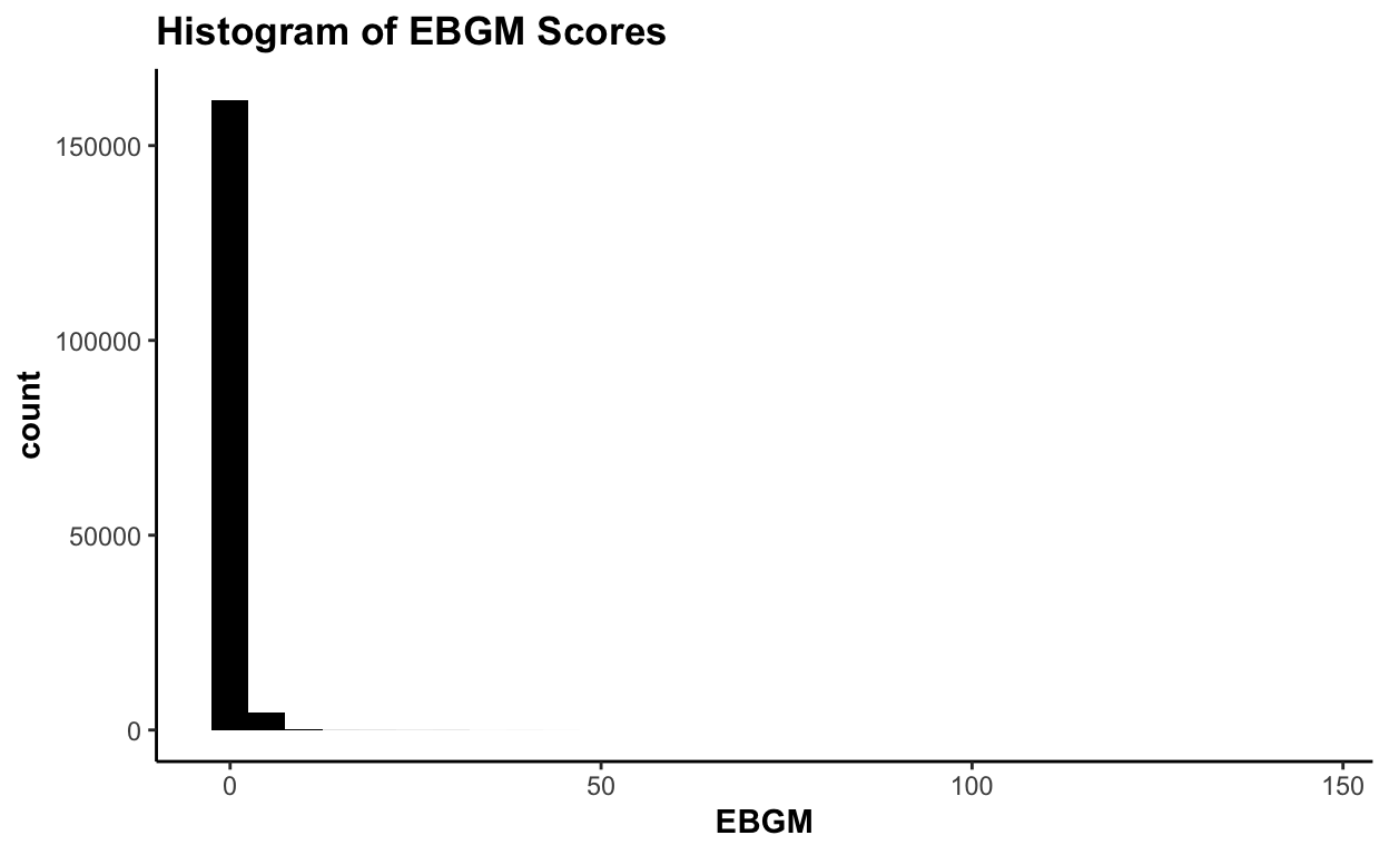
plot(ebout, plot.type = "shrinkage") + scale_color_nejm()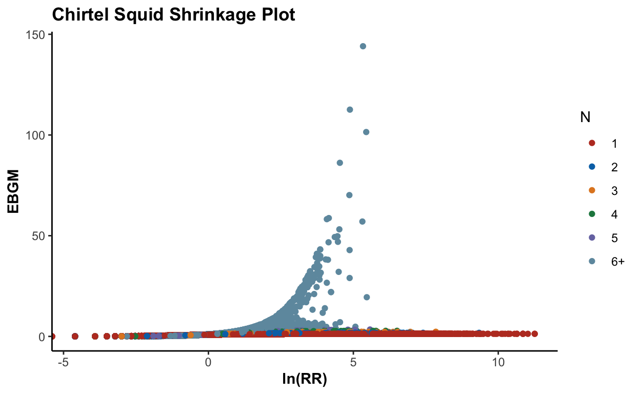
Let’s focus on a specific type of adverse event (vomiting):
plot(ebout, event = "Vomiting") + scale_fill_nejm()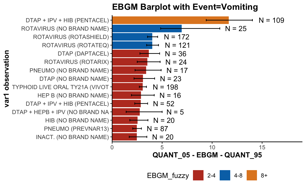
plot(ebout, plot.type = "histogram", event = "Vomiting")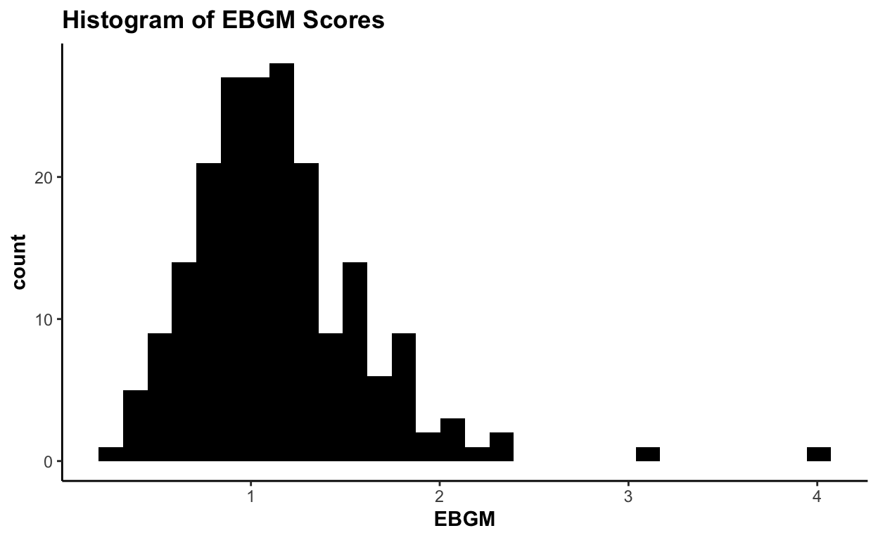
plot(ebout, plot.type = "shrinkage", event = "Vomiting") + scale_color_nejm()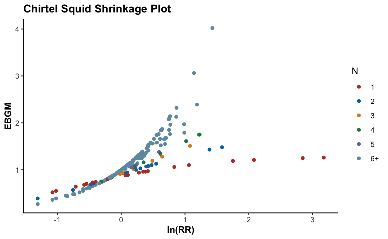
DuMouchel, William. 1999. “Bayesian Data Mining in Large Frequency Tables, with an Application to the Fda Spontaneous Reporting System.” The American Statistician 53 (3): 177–90.