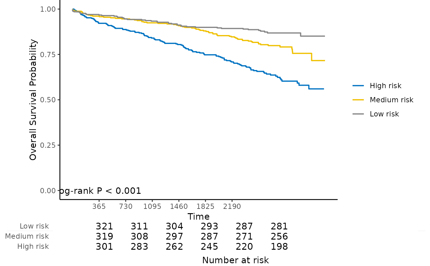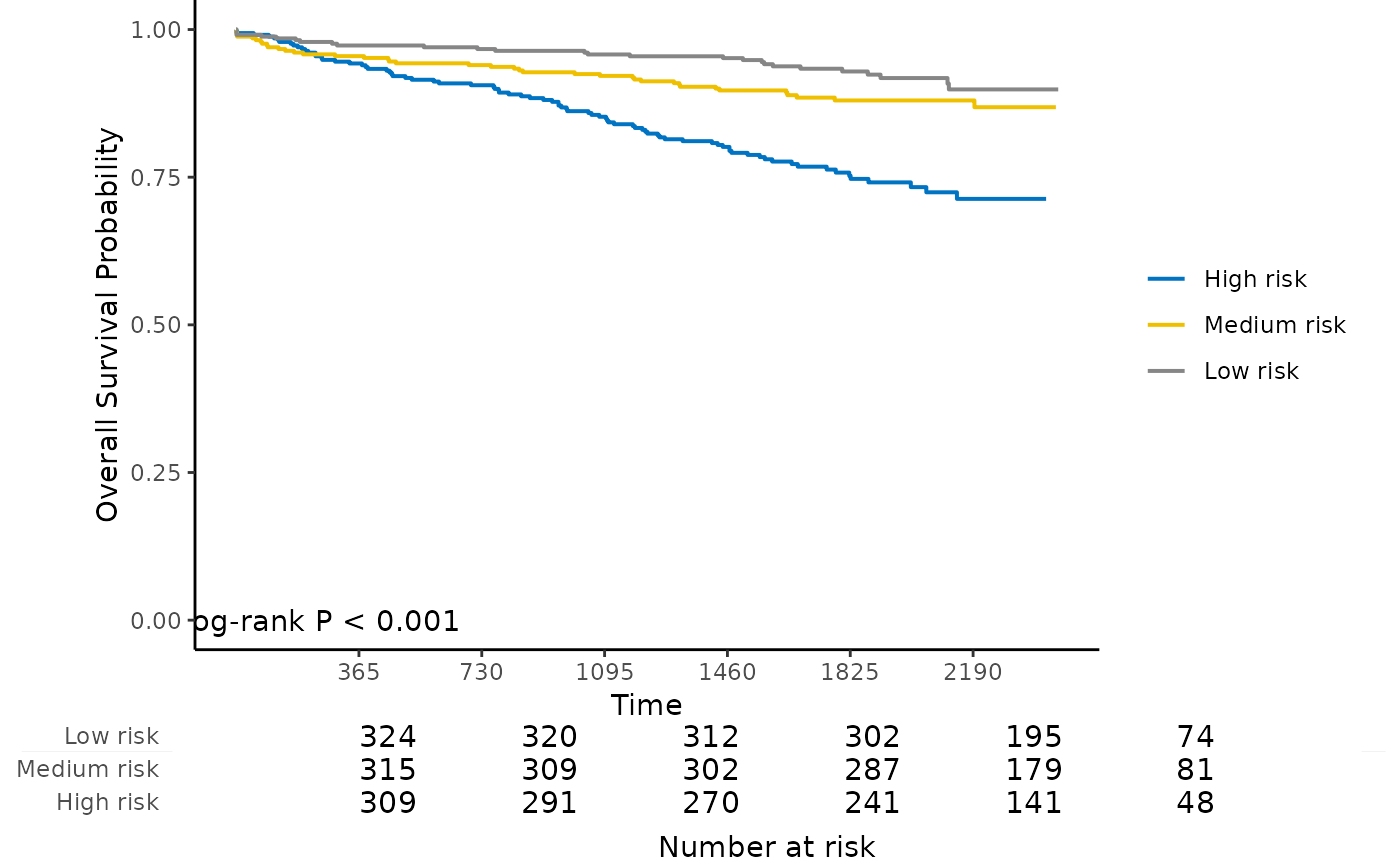
Kaplan-Meier plot with number at risk table for internal calibration and external calibration results

Usage

kmplot(
  object,
  group.name = NULL,
  time.at = NULL,
  col.pal = c("JCO", "Lancet", "NPG", "AAAS")
)

Arguments

object: An object returned by calibrate or calibrate_external.
group.name: Risk group labels. Default is Group 1, Group 2, ..., Group k.
time.at: Time points to evaluate the number at risk.
col.pal: Color palette to use. Possible values are "JCO", "Lancet", "NPG", and "AAAS". Default is "JCO".

Examples

data("smart")
# Use the first 1000 samples as training data
# (the data used for internal validation)
x <- as.matrix(smart[, -c(1, 2)])[1:1000, ]
time <- smart$TEVENT[1:1000]
event <- smart$EVENT[1:1000]

# Take the next 1000 samples as external calibration data
# In practice, usually use data collected in other studies
x_new <- as.matrix(smart[, -c(1, 2)])[1001:2000, ]
time_new <- smart$TEVENT[1001:2000]
event_new <- smart$EVENT[1001:2000]

# Fit Cox model with lasso penalty
fit <- fit_lasso(x, survival::Surv(time, event), nfolds = 5, rule = "lambda.1se", seed = 11)

# Internal calibration
cal.int <- calibrate(
  x, time, event,
  model.type = "lasso",
  alpha = 1, lambda = fit$lambda,
  method = "cv", nfolds = 5,
  pred.at = 365 * 9, ngroup = 3
)
#> Start fold 1 
#> Start fold 2 
#> Start fold 3 
#> Start fold 4 
#> Start fold 5 

kmplot(
  cal.int,
  group.name = c("High risk", "Medium risk", "Low risk"),
  time.at = 1:6 * 365
)


# External calibration
cal.ext <- calibrate_external(
  fit, x, time, event,
  x_new, time_new, event_new,
  pred.at = 365 * 5, ngroup = 3
)

kmplot(
  cal.ext,
  group.name = c("High risk", "Medium risk", "Low risk"),
  time.at = 1:6 * 365
)