Ensemble Partial Least Squares for Model Applicability Domain Evaluation

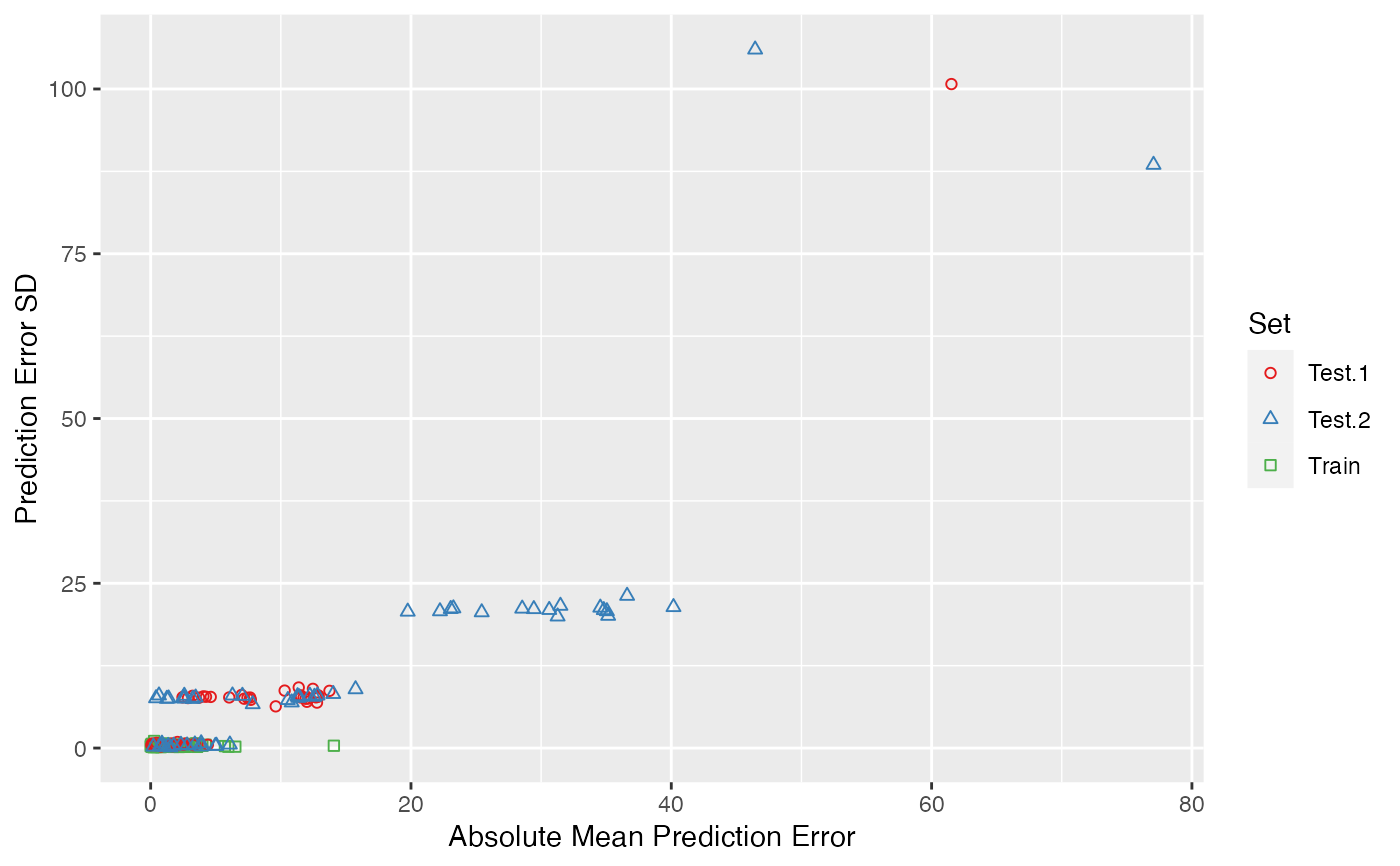
Model applicability domain evaluation with ensemble partial least squares.

Usage

enpls.ad(
  x,
  y,
  xtest,
  ytest,
  maxcomp = NULL,
  cvfolds = 5L,
  space = c("sample", "variable"),
  method = c("mc", "boot"),
  reptimes = 500L,
  ratio = 0.8,
  parallel = 1L
)

Arguments

x: Predictor matrix of the training set.
y: Response vector of the training set.
xtest: List, with the i-th component being the i-th test set's predictor matrix (see example code below).
ytest: List, with the i-th component being the i-th test set's response vector (see example code below).
maxcomp: Maximum number of components included within each model. If not specified, will use the maximum number possible (considering cross-validation and special cases where n is smaller than p).
cvfolds: Number of cross-validation folds used in each model for automatic parameter selection, default is 5.
space: Space in which to apply the resampling method. Can be the sample space ("sample") or the variable space ("variable").
method: Resampling method. "mc" (Monte-Carlo resampling) or "boot" (bootstrapping). Default is "mc".
reptimes: Number of models to build with Monte-Carlo resampling or bootstrapping.
ratio: Sampling ratio used when method = "mc".
parallel: Integer. Number of CPU cores to use. Default is 1 (not parallelized).

Value

A list containing:

tr.error.mean - absolute mean prediction error for training set
tr.error.median - absolute median prediction error for training set
tr.error.sd - prediction error sd for training set
tr.error.matrix - raw prediction error matrix for training set
te.error.mean - list of absolute mean prediction error for test set(s)
te.error.median - list of absolute median prediction error for test set(s)
te.error.sd - list of prediction error sd for test set(s)
te.error.matrix - list of raw prediction error matrix for test set(s)

Note

Note that for space = "variable", method could only be "mc", since bootstrapping in the variable space will create duplicated variables, and that could cause problems.

Author

Nan Xiao <https://nanx.me>

Examples

data("alkanes")
x <- alkanes$x
y <- alkanes$y

# training set
x.tr <- x[1:100, ]
y.tr <- y[1:100]

# two test sets
x.te <- list(
  "test.1" = x[101:150, ],
  "test.2" = x[151:207, ]
)
y.te <- list(
  "test.1" = y[101:150],
  "test.2" = y[151:207]
)

set.seed(42)
ad <- enpls.ad(
  x.tr, y.tr, x.te, y.te,
  space = "variable", method = "mc",
  ratio = 0.9, reptimes = 50
)
print(ad)
#> Model Applicability Domain Evaluation by ENPLS
#> ---
#> Absolute mean prediction error for each training set sample:
#>   [1]  1.15659310  0.37135659  0.18687002  1.17664393  0.12373621  1.00392170
#>   [7]  0.04434202  0.63828656  0.43718385  0.64726539  0.09051787  0.48966778
#>  [13]  3.62308256  0.52948567  0.25251989  3.32711614  0.95156004  0.14091017
#>  [19]  0.85464231  1.29109538  0.02019387  0.32245514  0.62770096  0.25487849
#>  [25]  0.46810576  0.67759188  0.25457816  0.69278642  0.70787689  0.72829569
#>  [31]  1.57186733  0.76802915  1.31022753  0.72248475  0.85636595  1.22138075
#>  [37]  0.45068514  1.40704563  1.21935389  1.11988622  2.19718455  2.45031644
#>  [43]  1.49666523  1.08541858  1.52751554  1.68620203  0.74572579  0.87057898
#>  [49]  2.03595023  1.89786907  1.68599205  0.05692682  3.87440488  0.97422048
#>  [55]  0.40778747  0.94140304  2.54484306  2.66435962  1.66527372  0.38685260
#>  [61]  0.92713783  3.58843757 14.16899449  5.94141096  0.84436844  1.12210481
#>  [67]  2.29468141  1.39277186  1.44998603  2.38993959  0.59566790  1.09886862
#>  [73]  1.27593299  2.05666549  1.63679051  2.12750518  0.27833880  1.85919482
#>  [79]  1.80079825  0.74364023  1.06912418  0.38683360  5.70973358  0.35817828
#>  [85]  2.67017284  0.71305049  2.17485482  2.01172042  1.54421445  0.26828780
#>  [91]  1.23313227  3.79410089  2.79472535  4.15099941  6.49989050  1.74711076
#>  [97]  3.54480005  1.57668886  1.79632988  1.09721925
#> ---
#> Prediction error SD for each training set sample:
#>   [1] 0.6723203 0.9925861 0.7916684 0.5353981 0.6833493 0.3750142 0.5384201
#>   [8] 0.4394781 0.4478961 0.3115000 0.2965013 0.6564925 0.8581624 0.6408359
#>  [15] 0.2112281 0.7276103 0.4012712 0.2924988 0.5139599 0.4312994 0.3225841
#>  [22] 0.2810618 0.3927624 0.3747409 0.2372358 0.4391011 0.4310893 0.2127917
#>  [29] 0.4711463 0.4231286 0.3089803 0.2203195 0.7273629 0.5681682 0.1253907
#>  [36] 0.1542993 0.5196908 0.4079485 0.3314376 0.2223870 0.6052788 0.2461725
#>  [43] 0.3104808 0.6333215 0.4917393 0.5680786 0.7958397 0.3688654 0.6318733
#>  [50] 0.4057159 0.3159804 0.3805643 0.7569301 0.3793449 0.1648608 0.3351091
#>  [57] 0.4672745 0.8267976 0.4487075 0.3364956 0.4968275 0.2133814 0.8887981
#>  [64] 0.2061471 0.2362712 0.5270498 0.2774651 0.3162993 0.5402216 0.4409003
#>  [71] 0.2945032 0.4952080 0.2839455 0.5987966 0.3229918 0.3881967 0.4959163
#>  [78] 0.5784472 0.2844325 0.8621228 0.4714674 0.1963147 0.2992360 0.4816676
#>  [85] 0.1823169 0.4285107 0.1955258 0.5412362 0.2689507 0.8016830 0.3348107
#>  [92] 0.4141135 0.6989277 0.5368645 0.2533462 0.1989506 0.3307565 0.7953010
#>  [99] 0.2301105 0.5033743
#> ---
#> Absolute mean prediction error for each test set sample:
#> [[1]]
#>  [1]  1.6168531  0.5129803  1.6250825  0.0203619  4.3383400  0.1106109
#>  [7]  0.8148653  1.9913556  3.2096770  2.2171926  2.5990837  2.6064094
#> [13]  3.3267257  1.5533525  0.2446492  2.7310229  3.3531130  0.6680140
#> [19]  1.9791727 12.2374458 13.4166499 11.1587762 14.5567185  8.4080822
#> [25] 10.1272429 10.6439947 13.7889019 12.3442711 12.6224187  7.7835221
#> [31]  4.2295455 12.6785692 12.9451491 13.7247623  5.0281196 13.6627983
#> [37] 12.7484447  5.1156233  3.4747344 13.4024321  6.8780031 12.3931679
#> [43]  5.5321643  3.3919701 13.4337748  8.3609657  4.5468609  3.7926681
#> [49]  8.4599080  7.8685360
#> 
#> [[2]]
#>  [1]  4.3639558  3.3964642 12.0544328 11.3324274  1.2463920  3.4669273
#>  [7]  2.2877420  8.5348824  2.0397521  0.3601160 38.9955576 33.2649875
#> [13] 37.2145440 33.8217957 37.3135529 31.7305484 42.5682817 37.0789591
#> [19] 25.5740117 28.1372472 31.0069656 25.5649259 27.7147261 37.1938925
#> [25] 33.1063600 24.4682094 22.2051201  0.2364423  1.0464166  3.5595735
#> [31]  2.7676125  2.3996208  1.7344534  0.7284600  6.1337782  1.5540024
#> [37]  5.0926006  5.2653924  0.7332907  1.3058880  4.0156528  1.0809554
#> [43]  4.9419237  0.7271527  3.9547319 16.5062741  3.9317236 15.0340504
#> [49]  3.5288351  7.1680305 13.2197061 11.5264492 12.0580371 13.5543787
#> [55]  8.0233824 13.7150370 12.3711093
#> 
#> ---
#> Prediction error SD for each test set sample:
#> [[1]]
#>  [1]   0.4797399   0.9133170   0.2210427   0.4467299   0.5539222   0.7202601
#>  [7]   0.3420715   0.4083844   0.7906344   1.3627053   0.8435695   0.6415281
#> [13]   0.8357520   0.9553027   0.8306586   0.8760966   0.6962081   1.5891505
#> [19]   1.0981642  12.2938695  12.2441362  11.7821422  11.3326666   9.8410896
#> [25]   7.9849343 376.9162082  11.1413626  10.5392662  10.4817856  10.3927164
#> [31]  11.0753343   9.4622277  10.1555745  10.7601625  10.8400841  10.0669724
#> [37]  10.0677476  10.2535897  10.6672633   9.0113683  10.2352971  10.4262657
#> [43]  10.3678646  10.4748206   9.7797714  10.3870910   9.8668577  10.2321430
#> [49]  10.0652508   9.5121937
#> 
#> [[2]]
#>  [1]  10.1638483  10.1759666   9.5177953   9.5385654   9.5055823   9.9554471
#>  [7]  10.0826334   8.5796991   9.4517702   9.3947894  30.8269969  26.2958694
#> [13]  26.7640324  28.8511638  27.9602633  28.0373320  28.6187614  29.0240439
#> [19]  27.9815166 359.7986836  28.5880154  28.7358163  27.3902084  27.9664479
#> [25]  28.3790335  27.1663120  27.9724002   0.2617093   1.4992584   1.3071739
#> [31]   0.5646261   0.4787582   0.3340600   0.6052250   0.7380154   0.3165511
#> [37]   0.4492955 384.6771020   0.2690984   0.4416264   0.8652585   0.1814238
#> [43]   0.3736143   0.3488580   0.9745984  11.3696246  10.2310526  11.3901862
#> [49]  10.9868325  10.5839028  11.0100009   8.9886192  10.0022008  10.6591029
#> [55]  11.0407728  10.8211976  10.5118858
#> 
plot(ad)

# the interactive plot requires a HTML viewer
if (FALSE) { # \dontrun{
plot(ad, type = "interactive")
} # }