Performs relevant component analysis (RCA) for the given data. It takes a data set and a set of positive constraints as arguments and returns a linear transformation of the data space into better representation, alternatively, a Mahalanobis metric over the data space.
The new representation is known to be optimal in an information theoretic sense under a constraint of keeping equivalent data points close to each other.
Arguments
- x
A
n * dmatrix or data frame of original data.- chunks
A vector of size
Ndescribing the chunklets:-1in thei-th place says that pointidoes not belong to any chunklet; integerjin placeisays that pointibelongs to chunkletj; The chunklets indexes should be1:number-of-chunklets.- useD
Optional. Default is
NULL: RCA is done in the original dimension andBis full rank. WhenuseDis given, RCA is preceded by constraints based LDA which reduces the dimension touseD.Bin this case is of rankuseD.
Value
A list of the RCA results:
B: The RCA suggested Mahalanobis matrix. Distances between data pointsx1,x2should be computed by(x2 - x1)^T * B * (x2 - x1).RCA: The RCA suggested transformation of the data. The data should be transformed byRCA * data.newX: The data after the RCA transformation.newX = data * RCA.
Details
The three returned objects are just different forms of the same output.
If one is interested in a Mahalanobis metric over the original data space,
the first argument is all she/he needs. If a transformation into another
space (where one can use the Euclidean metric) is preferred, the second
returned argument is sufficient. Using A and B are equivalent
in the following sense:
if y1 = A * x1, y2 = A * y2, then
(x2 - x1)^T * B * (x2 - x1) = (y2 - y1)^T * (y2 - y1)
Note
Note that any different sets of instances (chunklets),
for example, {1, 3, 7} and {4, 6}, might belong to
the same class and might belong to different classes.
References
Aharon Bar-Hillel, Tomer Hertz, Noam Shental, and Daphna Weinshall (2003). Learning Distance Functions using Equivalence Relations. Proceedings of 20th International Conference on Machine Learning (ICML2003).
Examples
library("MASS")
# Generate synthetic multivariate normal data
set.seed(42)
k <- 100L # Sample size of each class
n <- 3L # Specify how many classes
N <- k * n # Total sample size
x1 <- mvrnorm(k, mu = c(-16, 8), matrix(c(15, 1, 2, 10), ncol = 2))
x2 <- mvrnorm(k, mu = c(0, 0), matrix(c(15, 1, 2, 10), ncol = 2))
x3 <- mvrnorm(k, mu = c(16, -8), matrix(c(15, 1, 2, 10), ncol = 2))
x <- as.data.frame(rbind(x1, x2, x3)) # Predictors
y <- gl(n, k) # Response
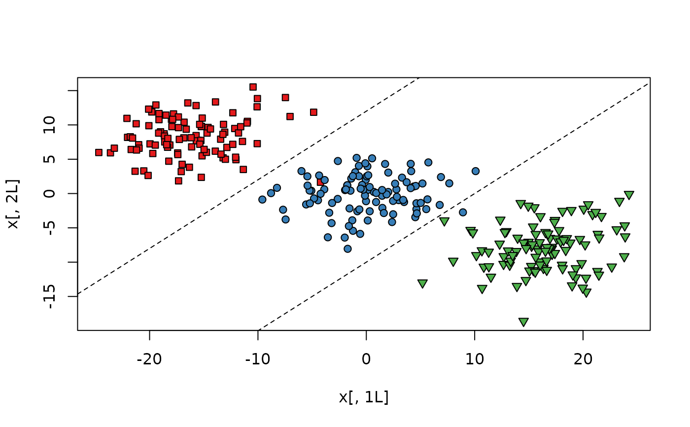
# Fully labeled data set with 3 classes,
# need to use a line in 2D to classify.
plot(x[, 1L], x[, 2L],
bg = c("#E41A1C", "#377EB8", "#4DAF4A")[y],
pch = rep(c(22, 21, 25), each = k)
)
abline(a = -10, b = 1, lty = 2)
abline(a = 12, b = 1, lty = 2)
 # Generate synthetic chunklets
chunks <- vector("list", 300)
for (i in 1:100) chunks[[i]] <- sample(1L:100L, 10L)
for (i in 101:200) chunks[[i]] <- sample(101L:200L, 10L)
for (i in 201:300) chunks[[i]] <- sample(201L:300L, 10L)
chks <- x[unlist(chunks), ]
# Make "chunklet" vector to feed the chunks argument
chunksvec <- rep(-1L, nrow(x))
for (i in 1L:length(chunks)) {
for (j in 1L:length(chunks[[i]])) {
chunksvec[chunks[[i]][j]] <- i
}
}
# Relevant component analysis
rcs <- rca(x, chunksvec)
# Learned transformation of the data
rcs$RCA
#> [,1] [,2]
#> [1,] -3.147411 -0.7864477
#> [2,] -1.026338 2.4117535
# Learned Mahalanobis distance metric
rcs$B
#> [,1] [,2]
#> [1,] 10.52470 1.333590
#> [2,] 1.33359 6.869925
# Whitening transformation applied to the chunklets
chkTransformed <- as.matrix(chks) %*% rcs$RCA
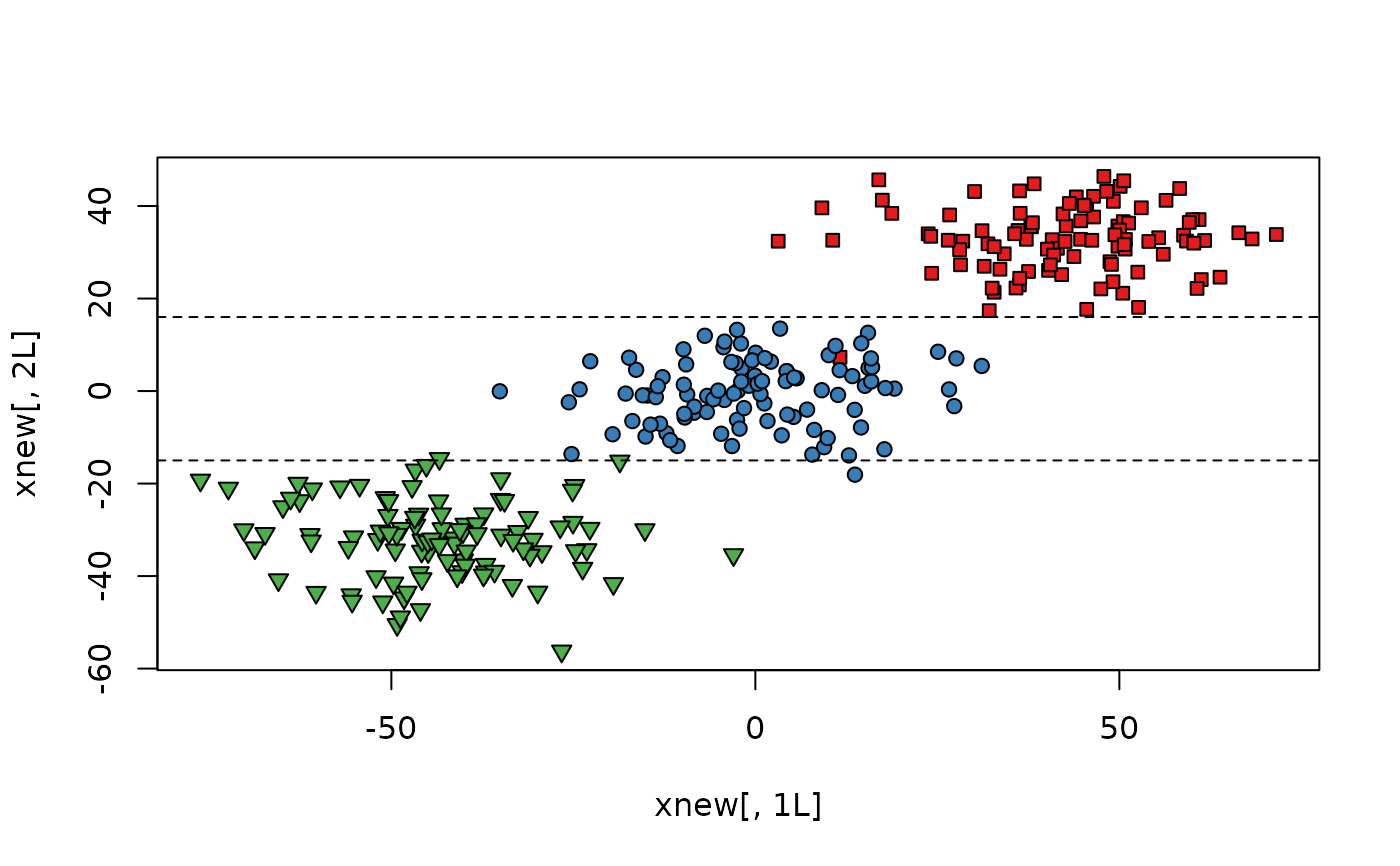
# Original data after applying RCA transformation,
# easier to classify - using only horizontal lines.
xnew <- rcs$newX
plot(xnew[, 1L], xnew[, 2L],
bg = c("#E41A1C", "#377EB8", "#4DAF4A")[gl(n, k)],
pch = c(rep(22, k), rep(21, k), rep(25, k))
)
abline(a = -15, b = 0, lty = 2)
abline(a = 16, b = 0, lty = 2)
# Generate synthetic chunklets
chunks <- vector("list", 300)
for (i in 1:100) chunks[[i]] <- sample(1L:100L, 10L)
for (i in 101:200) chunks[[i]] <- sample(101L:200L, 10L)
for (i in 201:300) chunks[[i]] <- sample(201L:300L, 10L)
chks <- x[unlist(chunks), ]
# Make "chunklet" vector to feed the chunks argument
chunksvec <- rep(-1L, nrow(x))
for (i in 1L:length(chunks)) {
for (j in 1L:length(chunks[[i]])) {
chunksvec[chunks[[i]][j]] <- i
}
}
# Relevant component analysis
rcs <- rca(x, chunksvec)
# Learned transformation of the data
rcs$RCA
#> [,1] [,2]
#> [1,] -3.147411 -0.7864477
#> [2,] -1.026338 2.4117535
# Learned Mahalanobis distance metric
rcs$B
#> [,1] [,2]
#> [1,] 10.52470 1.333590
#> [2,] 1.33359 6.869925
# Whitening transformation applied to the chunklets
chkTransformed <- as.matrix(chks) %*% rcs$RCA
# Original data after applying RCA transformation,
# easier to classify - using only horizontal lines.
xnew <- rcs$newX
plot(xnew[, 1L], xnew[, 2L],
bg = c("#E41A1C", "#377EB8", "#4DAF4A")[gl(n, k)],
pch = c(rep(22, k), rep(21, k), rep(25, k))
)
abline(a = -15, b = 0, lty = 2)
abline(a = 16, b = 0, lty = 2)